Weakly supervised learning for drowning detection in over-water construction from videos
*Correspondence to:
Yushu Yang, Department of Building and Real Estate, Hong Kong Polytechnic University, Hong Kong, China.
E-mail: ys-yushu.yang@connect.polyu.hk
J Build Des Environ. 2026;4:2025143. 10.70401/jbde.2026.0039
Received: December 23, 2025Accepted: May 06, 2026Published: May 08, 2026
This article belongs to the Special lssue Health and Safety Management in Construction: Innovations and Challenges
Abstract
Open-water drowning is a leading serious-injury/fatality risk at public waterfronts and in construction over or adjacent to water, where long stand-off views, glare, waves, and occlusions hinder timely detection. We propose TimeSformer+MIL, a weakly supervised temporal framework for event-level drowning monitoring designed for deployment in safety-critical construction settings and aligned with supervisory workflows. The system standardizes video streams into short clips, extracts spatiotemporal evidence with a divided space–time TimeSformer, and aggregates clip scores via top-k multiple-instance learning with a lightweight consistency prior to stabilize weak labels and support calibration. By avoiding person detection and multi-object tracking, the pipeline reduces engineering complexity and failure modes common in cluttered, low-light, or small-scale scenes, improving reliability without increasing operator load. We curate an open-water dataset spanning construction and public-waterfront contexts and evaluate with event-focused metrics aligned to risk governance: recall at target false-positives per hour, alert latency relative to rescue windows, and calibration-aware ranking and thresholded decisions for alerting and escalation. Across clip lengths and aggregation strategies, the approach delivers robust discrimination and translates it into stable, low-latency alerts that meet rescue-time targets while limiting alarm fatigue. For architectural practice and construction safety management, the framework offers a practical path to augment human surveillance with machine attention, functioning as a verifiable administrative control within the hierarchy of controls and integrating with site safety processes to accelerate incident recognition and strengthen risk governance in dynamic open-water settings.
Keywords
Drowning detection, open-water, TimeSformer, multiple instance learning, transformer-based video modeling, event-level evaluation
1. Introduction
Drowning in open waters is a serious construction safety hazard for work over or adjacent to water. According to a World Health Organization report, hundreds of thousands of people die from drowning each year, with open spaces such as beaches, rivers, and lakes being high-risk environments[1]. Beyond public recreation areas, water-related hazards are a persistent cause of severe and fatal incidents in construction and infrastructure operations, including marine construction, bridge and pier works, cofferdam and excavation near waterways, port logistics, and flood-control maintenance[2]. In these settings, workers are exposed to unstable footing, variable weather, and limited visibility, and rescue latency is a key determinant of survivability[3]. Regulatory frameworks reflect this reality: OSHA 29 CFR 1926.106 requires USCG-approved Personal flotation devices (PFDs), ring buoys (distance between ring buoys ≤ 200 ft; line length ≥ 90 ft), and an immediately available lifesaving skiff when employees work over or adjacent to water where a drowning danger exists; official interpretation letters further clarify that the skiff is required irrespective of continuous fall protection to ensure prompt rescue[4].Recent enforcement cases also underscore gaps between policy and practice, and high-profile infrastructure incidents have renewed scrutiny of on-water rescue readiness and communication during jobs over. Compared to indoor swimming pools, open waters are more significantly affected by tides, wind, and waves, visibility, crowding, and weather conditions. Traditional human patrols and fixed camera monitoring often suffer from limited coverage, restricted viewing angles, and high response latency, making it difficult to promptly detect and respond to sudden drowning incidents[5-7]. Furthermore, the scarcity of real drowning samples and the sensitive nature of annotations make constructing high-quality training datasets subject to ethical and privacy constraints, further exacerbating the uncertainty of algorithms in practical deployment.
Existing research has largely focused on controlled indoor swimming pool scenarios. In such environments, the water is clear, the lighting is stable, the background is simple, the camera’s viewing angle is fixed, and even underwater cameras are used, resulting in distinct human silhouettes and postures[8-11]. Taking advantage of these conditions, mainstream methods often employ motion analysis based on human posture or skeletons, or perform end-to-end classification across the entire video, achieving high accuracy in close-range imaging conditions with good visibility. However, these methods face significant challenges in portability, robustness, and usability in open water environments. High-frequency noise caused by surface reflections and wave spray, object fragmentation and keypoint loss due to floating objects and occlusions, the fact that people occupy only a few pixels when captured from a distance, and significant domain shift due to the diversity of devices and shooting angles all combine to weaken the effectiveness of pose estimation and whole-video classification. Furthermore, simple video-level binary classification struggles to output “which person and when” is drowning, thus failing to provide actionable alert information for rescue efforts.
In response to the challenges of open-water surveillance, we propose a temporally focused, instance-agnostic detection framework that emphasizes engineering feasibility and online usability. Methodologically, we adopt a single-stage temporal discrimination strategy: videos are standardized (frame rate, resolution) and segmented into short, overlapping clips; a TimeSformer-based classifier then produces clip-level drowning scores, which are aggregated with sliding windows and hysteresis to yield stable, low-latency alerts. This design eliminates dependency on prior object detection and multi-object tracking, reducing engineering complexity and failure modes in cluttered scenes, low light, occlusions, or small-scale targets. To further exploit weak supervision and reduce annotation burden, we cast training as a multiple instance learning (MIL) problem: each raw video (bag) comprises temporally segmented clips (instances), with only bag-level labels available for many samples[12,13]. We optimize the TimeSformer with MIL-style pooling over instance scores (e.g., max-/top-k/attention pooling) to align bag-level supervision with instance-level discrimination, while preserving the single-stage, detector-free pipeline. In practice, MIL pooling encourages the model to localize drowning-relevant segments within positive bags and to suppress spurious peaks in negatives, which directly benefits online stability and reduces false alarms. At the data level, we construct a standardized pipeline for open-media videos, including unified frames per second (FPS)/resolution, de-duplication and quality control, and segmentation into 10-30 s windows[14,15]. We adopt event-level weak supervision because confirmations are faster to obtain across sites and entail fewer privacy and liability concerns than frame- or box-level annotations. We implement this with top-k MIL and use semi-automatic candidate mining to mitigate the scarcity of positive samples and the cost of temporal annotations. To assess real-world value, we emphasize threshold-independent metrics at the event level (e.g., average precision (AP) and area under the ROC curve (AUC)) and characterize alert latency under the online hysteresis policy; we also report clip-/video-level precision-recall (PR)/AUC. We further compare system outputs with judgments from professional rescuers or experienced administrators to quantify operating trade-offs and to identify deployment-relevant failure modes.
The main contributions of this paper are as follows:
• We target the open-water gap where pool-trained frame classifiers break down. By casting monitoring as instance-level, time-series event detection, answering who and when, we handle tiny/distant targets and intermittent visibility (glare, waves, occlusion), and evaluate at the event level with latency and false-alarm budgets; the same design considerations echo those in construction-site safety where timely, low-FP alerts are critical.
• We deliver a deployable, instance-agnostic temporal framework: standardize streams; score short clips with a TimeSformer; aggregate via sliding windows and hysteresis to yield stable, low-latency alerts without object detection or multi-object tracking (MOT). This reduces engineering complexity and failure modes in cluttered, low-light, or small-scale scenarios, a practical trait for safety monitoring in dynamic, visually noisy environments (e.g., waterfronts or construction perimeters).
• We establish an open-media benchmark and data pipeline: event-level ground truth and metrics (recall, PR/AUC); unified FPS/resolution, de-duplication, and 10-30 s segmentation with weak-label mining. This supports reproducible comparisons and operational analysis, and the benchmarking rubric, event-level metrics at target operating points, translates naturally to adjacent safety domains such as construction for auditing and risk governance.
2. Literature Review
2.1 Indoor and outdoor drowning detection
With more sensing platforms now available, recent studies on drowning monitoring can be grouped into four observation regimes: pool-focused vision, vision in natural waters, aerial views from unmanned aerial vehicles (UAVs), and non-visual channels. In pools, cameras above or below the waterline typically encode signs of distress as partially visible bodies near the surface, upright postures, and proximity to lanes or geofenced zones—conditions that benefit from short viewing ranges and stable lighting[5,6,10,11,16]. In natural settings such as beaches, rivers, or offshore areas, cues shift toward brief head/arm glimpses under long stand-off, strong glare, waves, and frequent occlusions, so methods rely more on robust spatio–temporal evidence from local parts[7,17,18]. UAV-based work adds top-down, wide-area coverage for rapid search and triage[19]. Beyond vision, several threads target “distress intent” or physiological proxies: radio frequency identification (RFID) wearables that fall silent during prolonged submersion, multi-sensor bands that fuse oxygen/respiration/immersion signals, underwater acoustic save our souls (SOS) detection from commodity devices, and yarn-based strain/flow sensors that emit coded alerts on water entry[9,20-22]. Taken together, these regimes span a cue continuum from appearance near the water surface to explicit distress signals and physiological markers.
2.2 Vision-based drowning detection method
Most vision pipelines start from single-frame detectors and adapt them to water scenes. Variants of the YOLO family (v5/v7/v8/v11) are common, pairing lightweight convolutions (e.g., Ghost or dynamic forms), attention-style modules, and revised feature pyramids (e.g., BiFPN-like bidirectional fusion) to balance accuracy, speed, and embedded deployment[5,6,11,17,18,23]. In crowded lanes or multi-swimmer scenes, deformable operations, auxiliary heads, and loss redesign sharpen the boundary between “swimming” and “drowning” under clutter[8]. Two-stage designs also appear: a light detector flags human candidates (often near-vertical poses), followed by a compact verifier to meet real-time limits on embedded boards[10]. For natural waters, methods emphasize small-object sensitivity and occlusion robustness, combining activation replacements (e.g., FReLU), conv–self-attention hybrids, refined IoU losses, and structured pruning to sustain performance at distance while improving FPS[7]. In parallel, nonvisual approaches treat events as thresholded states or learned detections in RFID/wearable or underwater-acoustic streams[9,20,21]. Synthetic data has been explored to enrich rare appearances and hard cases[8]. Overall, the field leans toward efficient detectors with water-aware modules, wrapped in pipelines that trade modest complexity for practical latency and deployment.
Modern detector-based systems (e.g., YOLO variants) perform strongly in controlled, short-range views. Performance can degrade in long-range scenes with glare, heavy occlusion, and spray when detections or associations become unstable, and errors at the detection stage propagate to downstream alert logic. Our instance-agnostic temporal formulation avoids this dependency and simplifies the deployment pipeline, so we focus comparisons on clip-level temporal classifiers rather than detector–tracker stacks.
2.3 Data sources and evaluation protocols
Across the literature, a typical data path emerges: controlled pools, often with underwater or near-wall viewpoints and staged behaviors, followed by selective forays into natural waters or UAV imagery. Many pool studies build self-collected sets under stable light and short ranges, with volunteers enacting variants of the instinctive drowning response or proxy motions (e.g., ladder-climbing, back-float/backstroke) to increase class separability[5,11,23]. Embedded constraints are considered in some works, targeting real-time on devices such as Jetson Nano or Raspberry Pi[6,10]. Natural-water and offshore efforts rely on bespoke collections or task-specific corpora to capture distant, small targets and cluttered backgrounds, while UAV data extends area coverage[7,17-19].
This data ecology exposes two structural limits for open-water use and for “data truthfulness”. First, the domain gap: illumination statistics, specular highlights, wave patterns, occlusion rates, viewing geometry, and crowd density differ markedly between pools and open waters, so models trained on controlled, short-range imagery may not generalize reliably. Second, the action source: staged episodes by cooperative volunteers, bounded by ethics and safety, need not match the timing, surfacing rhythm, or partial-visibility patterns of real, non-cooperative incidents, which weakens event-level validity and claims about alert timeliness[6,23]. Synthetic imagery can diversify appearances, but its distributional fidelity to real open-water incidents remains to be established against in-situ benchmarks[8]. These observations motivate datasets that prioritize authentic open-water scenes, cross-domain splits, and event-level reporting (e.g., detection latency and false alarms per hour), so algorithmic gains translate into reliable alerting in the wild.
3. Methodology
We adopt a consistent notation throughout. Table 1 summarizes all symbols used in this section.
Table 1. Notation used in the methodology (kept only for components implemented in our training code).
| Symbol | Description | Default/Range |
| V = {Ft}Nt=1 | A video as a frame sequence | - |
| N | Total number of frames in V | - |
| K | Number of temporal segments (clips) in V | Ktrain = 4, Kval = 8 |
| T | Frames per clip | {8,16} |
| Ck | k-th clip, Ck = {FIk,i}Ti=1 | - |
| Φθ | TimeSformer encoder (divided space-time) | - |
| hk ∈ RD | Clip representation (backbone output) | - |
| yk | Logit for clip k (pre-sigmoid) | - |
| sk | Calibrated probability sk = σ(yk/τ) | - |
| τ | Temperature for calibration, τ = max{1, exp(ℓτ)} | learned |
| yV | Video-level label (weak supervision) | {0,1} |
| kMIL | MIL top-k size for a bag with NV clips | kMIL = [kratioNV] |
| kratio | MIL top-k ratio | 0.2 |
| λ | Weight of the consistency term | 0.1 |
3.1 Framework overview
Figure 1 presents the overall workflow: standardized decoding and clip sampling, TimeSformer encoding, top-k MIL with a small L1 consistency prior for stable supervision, and validation on ROC-AUC/AP. This design parallels deployment, where clip scores are aggregated by a short sliding window and a two-threshold hysteresis to convert discrimination into low-latency, stable alerts. Starting from a JSON list {path,label}, we decode each video with Decord and partition it into K equal-length temporal segments. Within the k-th segment we sample T frames to form a clip Ck. Let the segment boundaries be
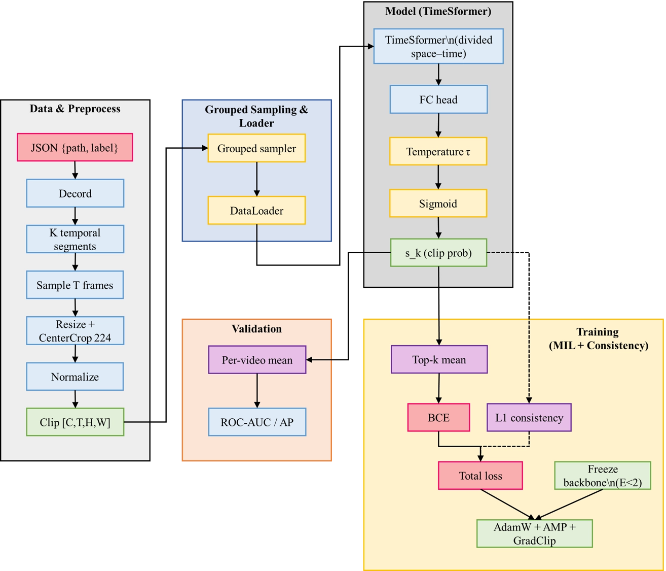
Figure 1. Training and validation workflow. MIL: multiple instance learning; AUC: area under the ROC curve; AP: average precision; FC: fully connected; ROC: receiver operating characteristic.
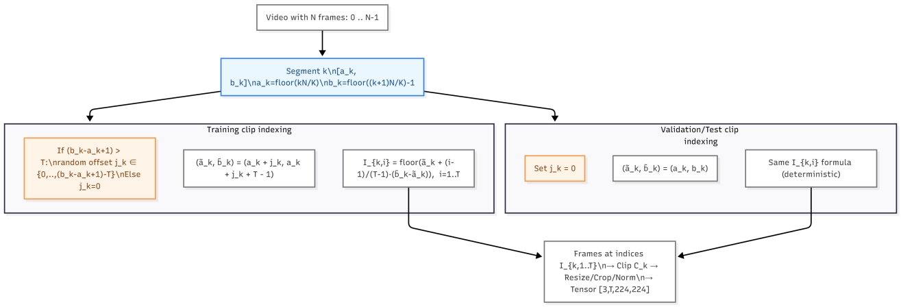
and validation/testing use the deterministic choice jk = 0 Figure 2 illustrates the segment-based clip construction and the uniform indexing defined in Eq. (1). Frames are resized by scaling the shorter side to 224 while preserving aspect ratio, then center-cropped to 224*224 and normalized by ImageNet mean/std; clips are fed as [C, T, H, W] tensors. A TimeSformer Φθ with divided space–time attention encodes each clip and a single fully-connected head outputs a logit yk:
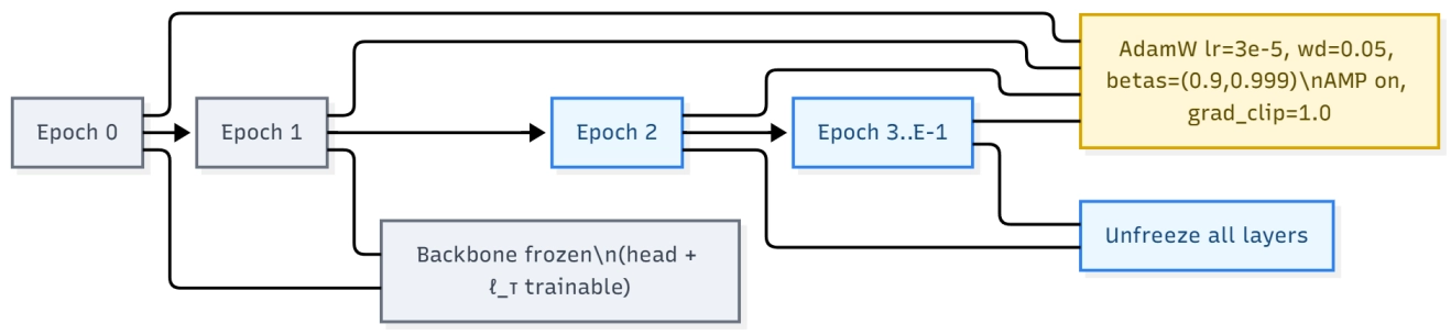
where σ(∙) is the sigmoid. We learn a temperature τ = max{1, exp(ℓτ)} end-to-end to calibrate probabilities; in practice we clamp τ ≥ 1 during training and inference. To stabilize weak supervision, we employ a video-grouped batch sampler that packs multiple clips from the same video while limiting the number of distinct videos per minibatch (default one video per batch). We also freeze the backbone for the first two epochs before unfreezing all layers, and train with AdamW (lr 3 × 10⁻⁵, weight decay 0.05, betas (0.9, 0.999)), mixed precision, and gradient clipping of 1.0. The warm-up, freezing/unfreezing schedule, and optimization settings are summarized in Figure 3.
Ablation During online inference, the model emits a probability sk for each incoming clip. A short sliding window aggregates these probabilities into a stream score. A two-threshold hysteresis policy turns the alert on when the score exceeds a higher threshold and releases it only after falling below a lower threshold, which suppresses chattering under glare and wave noise. Top-k multiple-instance pooling concentrates supervision on salient segments during training, shortening the time needed to accumulate sufficient evidence at test time. The expected trigger delay is on the order of one clip plus the window stride and remains compatible with low-latency requirements.
3.2 Learning from weak video labels
Divided space–time attention aggregates weak spatial cues across patches within a frame and integrates them over adjacent frames. Partial observations such as brief head or arm glints are intermittent under occlusion, glare, and spray. By first attending within-frame and then across time, the mechanism collects these fragments into a coherent pattern without relying on persistent detections or identity tracking. This reduces sensitivity to lost tracks and improves recall for tiny, distant targets.
With only a video-level label yV ∈ {0,1}, we aggregate clip probabilities within each video bag using a top-k mean. An overview of the weak-supervision pipeline, including the grouped sampler and top-k aggregation, is shown in Figure 4. For a video V with NV clips, let kML = [kratioNV] and IV be the indices of the kML largest {Sk}. The bag score and video-level loss are
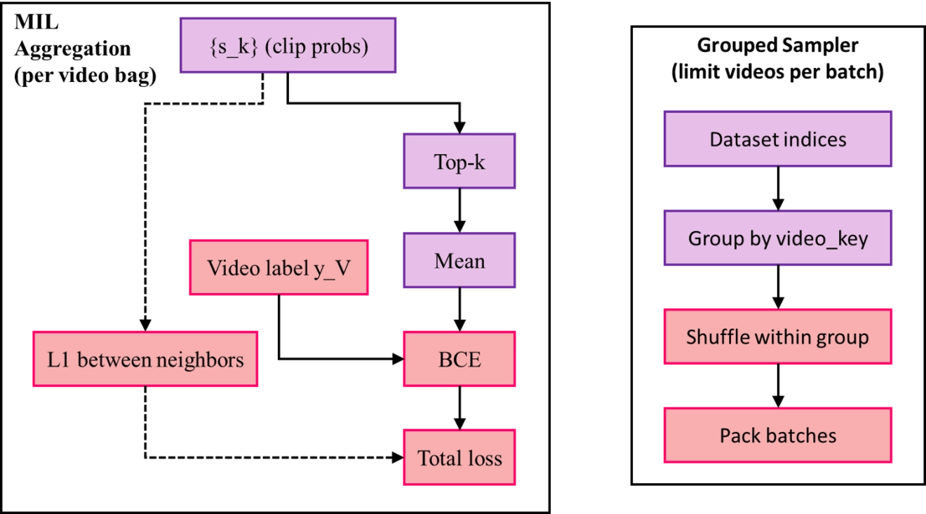
Figure 4. Weak-supervision pipeline with grouped sampler. MIL: multiple instance learning; BCE: binary cross entropy.
To discourage spurious fluctuations within a video, we impose an L1 consistency penalty on adjacent clip probabilities inside each bag (adjacent here follows the in-batch order of clips from the same video produced by the grouped sampler):
Where B indexes videos present in the current mini-batch. The training objective is the weighted sum
with kratio = 0.2 and λ = 0.1 unless stated otherwise. During validation, clip probabilities belonging to the same video are averaged to obtain a bag-level score for computing ROC-AUC and AP.
On the consistency weight λ. We use a small weight on the L1 consistency term to attenuate high-frequency score jitter between adjacent clips rather than to enforce long transitions. Because the online alert policy employs a two-threshold hysteresis at inference (Section 3.1), sensitivity to sudden onsets is preserved, the trigger threshold is unchanged. On the validation split, reduced jitter coincides with stable or improved AP and AUC, suggesting no loss of responsiveness.
3.3 Experiments
3.3.1 Implementation details
Experiments were conducted on a Windows 11 64-bit system equipped with an Intel(R) Core(TM) i5-14400F (16 CPUs), 32GB of system memory, and an NVIDIA GeForce RTX 4060 Ti GPU with 8GB of VRAM. All models in this study were written in Python 3.10, using the PyTorch 2.5.1 deep learning framework and torch.amp mixed precision. Unless otherwise noted, we trained at 6 fps, using segments of length T = 8 and stride s = 4, and resized frames to 224 × 224 while maintaining the aspect ratio. We used AdamW as the optimizer and selected the checkpoint with the best validation ROC-AUC.
3.3.2 Building of dataset
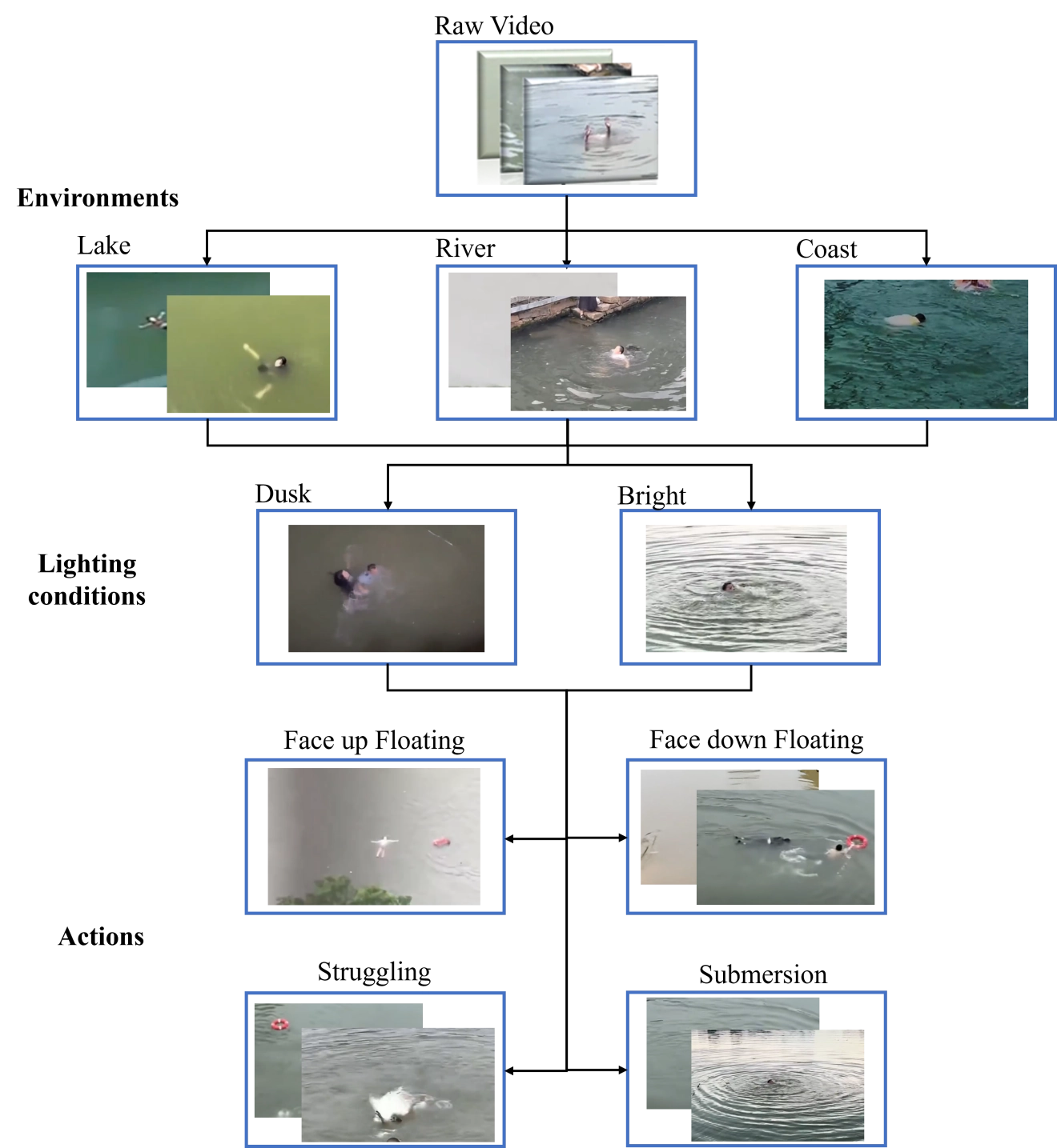
Deep learning methods for drowning detection require large, diverse, and carefully annotated datasets, yet existing swimming or action datasets largely capture general swimming behaviors and are dominated by pool scenes; to the best of our knowledge, no dedicated dataset targets drowning incidents in open water. To bridge this gap, we curate a dataset built from real-world recordings rather than simulations, since staged data often fails to reproduce the dynamics and visual ambiguity of genuine incidents. We search social media, video-sharing platforms, and news reports for videos in which a drowning event or a clearly non-drowning activity is visibly present, prioritizing authenticity and removing low-quality or unstable clips. An overview of the data collection is provided in Figure 5. The collected material spans varied open-water conditions, including lakes, rivers, reservoirs, and near-coastal areas, under diverse illumination and weather; it also covers challenging visual factors such as water glare, surface reflections, waves, occlusions, camera motion, and compression artifacts. For positive samples, we include representative behaviors such as face-down floating, back-floating with limited control, vertical struggle without effective forward motion, intermittent submergence, and periods with minimal or no motion; for negative samples, we include normal swimming, floating, treading water, playful splashing, and resting near shore without distress. Each retained clip is screened to ensure unambiguous class identity, low-quality footage is discarded, and annotators record a clip-level label (drowning vs. non-drowning) with approximate start–end times of the key event when available; optional contextual tags such as water type, lighting, weather, camera type, and viewpoint are also encouraged to support analysis. We term the resulting collection the Open-Water Drowning Incident Video dataset, short name: ODIV. After filtering and consolidation, ODIV contains 101 positive samples (drowning incidents) and 102 negative samples (normal swimming or non-distress activities), with clip durations ranging from roughly 10 seconds to several minutes. To promote reliable use, we recommend clear ethics and privacy handling (face/PII blurring and compliance with platform terms), transparent licensing or re-download scripts when redistribution is restricted, subject- and scene-disjoint train/validation/test splits to prevent leakage, double-annotation with conflict resolution and reported inter-annotator agreement, and baseline task definitions for clip-level classification and temporal localization with metrics such as AUC, AP, and F1, while emphasizing that automated detection should augment, not replace, human supervision in safety-critical settings. We use 224 × 224 crops to sustain throughput and reduce overfitting in a small data regime. Dense temporal sampling and spatiotemporal attention compensate for limited spatial detail by integrating weak cues across time.
3.3.3 Evaluation metrics
We evaluate clip-level drowning detection as a binary classification task and report accuracy, precision, recall, F1, and AP. Accuracy measures the fraction of correct predictions. Precision and recall quantify performance on the positive class, and their harmonic mean is summarized by the F1 score. To account for the choice of decision threshold, we sweep the threshold over [0,1], compute the precision–recall curve, and report AP as the area under this curve. Because our main task is binary and we report a single AP for the drowning class, mean average precision (mAP) is not required; mAP would be used only if we averaged AP across multiple classes or across multiple overlap thresholds in a temporal localization setting.
where TP, TN, FP, and FN denote the numbers of true positives, true negatives, false positives, and false negatives, respectively, computed on a given split. Precision and recall are defined with respect to the positive (drowning) class unless otherwise stated. For AP, let p(r) be the precision as a function of recall r [0,1] obtained by sweeping the decision threshold over the model’s confidence scores; AP is the area under this precision–recall curve. When reporting mAP (not used as a primary metric here), AP is averaged across classes or evaluation settings as specified. All metrics are reported on the held-out test set, with thresholds selected on the validation set.
We report threshold-independent metrics, including AP and AUC, and we use an event-level F1 score under a validated operating point selected on the validation split. In contrast, false positives per hour (FP/h) depend on the chosen decision threshold, the online hysteresis policy, and the amount of negative footage. Under the present dataset and protocol, these factors preclude a reliable FP/h estimate, so FP/h is not reported here. Quantitative FP/h is deferred to deployment studies and future releases where operating thresholds, hysteresis settings, and exposure to negative hours are controlled and auditable.
3.3.4 Data splits
We partition the dataset into three disjoint splits to support model development and unbiased evaluation. As summarized in Table 2, the training set contains 74 positive and 68 negative clips (142 total), the validation set contains 18 positive and 22 negative clips (40 total), and the test set contains 9 positive and 13 negative clips (22 total), for an overall total of 101 positive and 102 negative clips (203 total). To characterize the data beyond counts, Table 3 reports the composition across open-water types (lake, river, coastal, and mixed/unknown), and Table 4 summarizes viewing and recording conditions (bright, dusk/night, backlight/glare). Splits are constructed to be subject- and scene-disjoint whenever identifiable, avoiding leakage across the same incident or location. Class balance is kept approximately even to stabilize optimization and threshold selection, with the validation set used exclusively for hyperparameter tuning and early stopping and the test set reserved for final reporting. All preprocessing, filtering, and de-duplication are performed prior to splitting, and clips with ambiguous labels are removed, ensuring that subsequent results reflect generalization rather than memorization under a fixed, reproducible split.
Table 2. Summary statistics of the dataset by split (clip counts only).
| Split | Pos (#clips) | Neg (#clips) | Total (#clips) |
| Train | 74 | 68 | 142 |
| Val | 18 | 22 | 40 |
| Test | 9 | 13 | 22 |
| All | 101 | 102 | 203 |
Table 3. Distribution across open-water types. Percentages are over all 203 clips.
| Category | Pos | Neg | All | % of All |
| Lake | 44 | 62 | 106 | 52.2% |
| River | 32 | 26 | 58 | 28.6% |
| Coastal | 13 | 14 | 27 | 13.3% |
| Mixed/Unknown | 12 | 0 | 12 | 5.9% |
| Total | 101 | 102 | 203 | 100.0% |
Table 4. Distribution across viewing/recording conditions. Percentages are over all 203 clips.
| Condition | Pos | Neg | All | % of All |
| Bright | 88 | 91 | 179 | 88.2% |
| Dusk/Night | 7 | 3 | 10 | 4.9% |
| Backlight/Glare | 6 | 8 | 14 | 6.9% |
| Total | 101 | 102 | 203 | 100.0% |
3.3.5 Standardized preprocessing and slicing
To ensure consistent training and evaluation on open-water footage, we employ a standardized pipeline that performs link- and fingerprint-based deduplication and discards unplayable or corrupted files. Videos are decoded via uniform frame indexing (independent of native FPS). Frames are resized by scaling the shorter side to 224 pixels while preserving aspect ratio, then center-cropped to 224 × 224, and normalized with ImageNet statistics (mean [0.485, 0.456, 0.406], std [0.229, 0.224, 0.225]). Each video is divided into K equal temporal segments; within each segment we uniformly sample T frames to form a clip. During training we use a random offset inside each segment to increase diversity, while validation/test use deterministic uniform sampling. Segments typically cover 10-30 seconds of context so that each clip contains pre-event and post-event evidence; for very short footage we mirror/loop frames to satisfy the frame count. Audio is removed by default, and when detachable subtitles or watermark layers are present we record their spatial regions as metadata for subsequent occlusion annotation and confidence analysis. Unless otherwise stated, we set K = 4 for training and K = 8 for validation/test, matching the implementation.
3.3.6 Implementation details and experimental setup
Our model is the official TimeSformer with divided space–time attention; we replace the classification head with a single logit for binary prediction. Let a video v be partitioned into Nv clips (instances). The network outputs a logit zv,i per instance; we apply a learnable temperature τ = exp(log_tau) and obtain calibrated probabilities
where σ(∙) is the sigmoid. Training follows MIL with a top-k mean aggregator. With kv = [αNv] and α ∈(0,1) (we use α = 0.2), let Iv be the indices of the kv largest pv,i; the bag score is
We supervise at the video level with binary cross-entropy,
and encourage temporal smoothness by penalizing adjacent instance-score differences,
The total loss is
Optimization uses AdamW with learning rate 3 × 10⁻⁵, weight decay 0.05, and (β1, β2) = (0.9,0.999). We train for 10 epochs with mixed precision and gradient clipping of 1.0. The backbone is frozen for the first two epochs and then unfrozen. Mini-batches are built by a video-grouped sampler that packs multiple clips from the same video while limiting the number of distinct videos per batch, which stabilizes MIL optimization. Unless otherwise specified, the input is 224 × 224 with T frames per clip (set according to the ablation), batch size is 8, and the random seed is 42. At evaluation, clip probabilities of the same video are averaged to obtain a bag-level score
3.3.7 Ablation studies
We study design choices under the same training protocol on the validation split and then fix the best setting for all main comparisons. First, we vary the temporal window length by sweeping T ∈ {8, 16, 32} and measure its effect on clip-to-video performance; if T = 16 yields the highest validation AP/AUC, we adopt T = 16 as the default for all subsequent experiments and report improvements as ∆AP(T) = AP(T) - AP(Torig). Next, we probe MIL hyperparameters by changing the top-k ratio α ∈ {0.1, 0.2, 0.3} and the consistency weight λ ∈ {0, 0.05, 0.1, 0.2} in Eqs. (12)-(15); the goal is to balance sensitivity to salient instances with temporal stability. Finally, we compare the video-grouped sampler to a naive shuffled sampler and toggle the training offset (random vs. deterministic) to assess their influence on validation metrics and optimization stability. All ablations keep data splits, preprocessing, optimizer, schedule, and all other settings unchanged to ensure fair attribution to the factor under study, and the configuration selected here is used in the Results section for external comparisons.
3.3.8 Comparative experiment design
We conduct a controlled comparative experiment to evaluate the proposed method against three baselines implemented in our code: I3D[24], convolutional neural network-long short-term memory (CNN-LSTM) [25,26], and TimeSformer without MIL (noMIL)[16-18]. The goal is to attribute performance and efficiency differences solely to model design while holding all other factors constant. All methods use the same binary video classification setup (drowning vs. non-drowning), the same train/val JSON splits, identical frame sampling, preprocessing, loss, optimization, and evaluation code paths. For each video we uniformly sample T frames; short videos use boundary repetition. Frames are center-cropped to square if needed, resized (e.g., 224), normalized with ImageNet statistics, arranged channels-first, and fed without content changes (only axis permutation when required). T and input resolution are matched across methods; batch size is kept the same whenever memory allows, otherwise we reduce only the batch and record it. Training uses AdamW (lr = 3e-4, wd = 0.05), fixed epochs (e.g., 30), the same schedule (or fixed LR), AMP enabled, and BCEWithLogitsLoss; if the main pipeline applies class weights or focal loss for imbalance, the same setting is applied to all models. Early stopping/model selection follow the same validation criterion (e.g., best AP or AUC) and tie breaking. Pretraining policy is aligned across methods (all use available pretraining or none); unavoidable mismatches are noted while keeping everything else unchanged. Architectures follow our implementations: I3D as an inflated 3D ConvNet with a single-logit head on [B,3,T,H,W] inputs[24]; CNN-LSTM with a framewise 2D CNN (e.g., ResNet-50) feeding a 1-2 layer LSTM (hidden 512/1024), using the final hidden state and a 1D head[25,26]; TimeSformer (noMIL) with decomposed spatiotemporal attention, aligned patch size/resolution/T, trained with video-level supervision on the CLS token and no MIL or instance pooling. The proposed model is trained in the same pipeline, changing only the modeling component. Validation uses the same sampler and center-crop; we report ROC-AUC and AP as primary metrics and Accuracy/F1 at a single threshold chosen by the same rule for all methods (e.g., max F1 on val), using the same search procedure. Efficiency is measured under identical conditions (same hardware, AMP on, same dataloader workers), reporting throughput (clips/s) and peak memory; if a method needs a smaller inference batch, we use its maximal feasible batch and document it. We fix the global seed (42), log software versions, and ensure identical code paths, thereby isolating modeling effects for a fair comparison between I3D, CNN-LSTM, TimeSformer (noMIL), and the proposed method.
4. Results
4.1 Main results on the test set
On the held-out test set, Ours (TimeSformer+MIL) attains Accuracy, AP, and AUC 0.975. The validation AUC/AP trajectories are summarized in Figure 6. To contextualize these results, we train a divided space-time TimeSformer with 8-frame 224 × 224 inputs and ImageNet/Kinetics pretraining on 142 training videos (74/68 pos/neg) and validate on 40 videos (18/22) with zero split overlap, using AdamW (lr 3 × 10⁻⁵, wd 0.05) under mixed precision and a two-epoch warm-up with the backbone frozen. Over a 60-epoch schedule (indices 0-59), validation AUC/AP rise quickly during warm-up (Epoch ; Epoch and jump sharply once the backbone is unfrozen at Epoch 2 (AUC 0.980; AP). The best validation checkpoint is reached early at Epoch 5 with AUC 0.992 and AP. Thereafter, performance remains high: from Epoch 2 onward AUC typically stays in the 0.96-0.98 band and AP in the 95-98% band, with a few transient dips (e.g., Epoch 24: AUC 0.949, AP 89.6% Epoch 30: AUC 0.942, AP 92.3%; Epoch 35: AUC 0.939, AP 93.2%), followed by rapid recoveries (e.g., Epoch 38: 0.982/97.5%; Epoch 43:0.982/98.0% and a strong ending at Epoch 58 (0.965/96.1%). The loss curves (Figure 7) track these dynamics: the bag-level cross-entropy (mil_bce) starts high and briefly spikes when unfreezing (0.850 at Epoch 2) before decaying to near-zero values (as low as 1 × 10⁻⁴ around Epoch 44), while the consistency regularizer (mil_cons) steadily decreases from ≈0.095 to 1.6 × 10⁻³ by the end, indicating improved temporal smoothness rather than overfitting to isolated clips. Precision–recall behavior at a fixed threshold (t = 0.5; Figure 8) shows precision stabilizing around 90-95% with occasional recall dips in the early-30s epoch range, after which both recover and maintain a high F1. The complementary loss and precision–recall analyses are shown in Figure 7 and Figure 8.
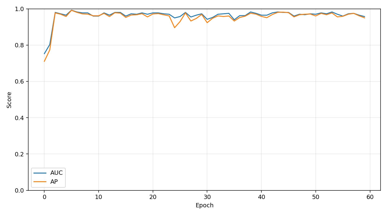
Figure 6. Validation performance curves (AUC & AP). AUC: area under the ROC curve; AP: average precision.
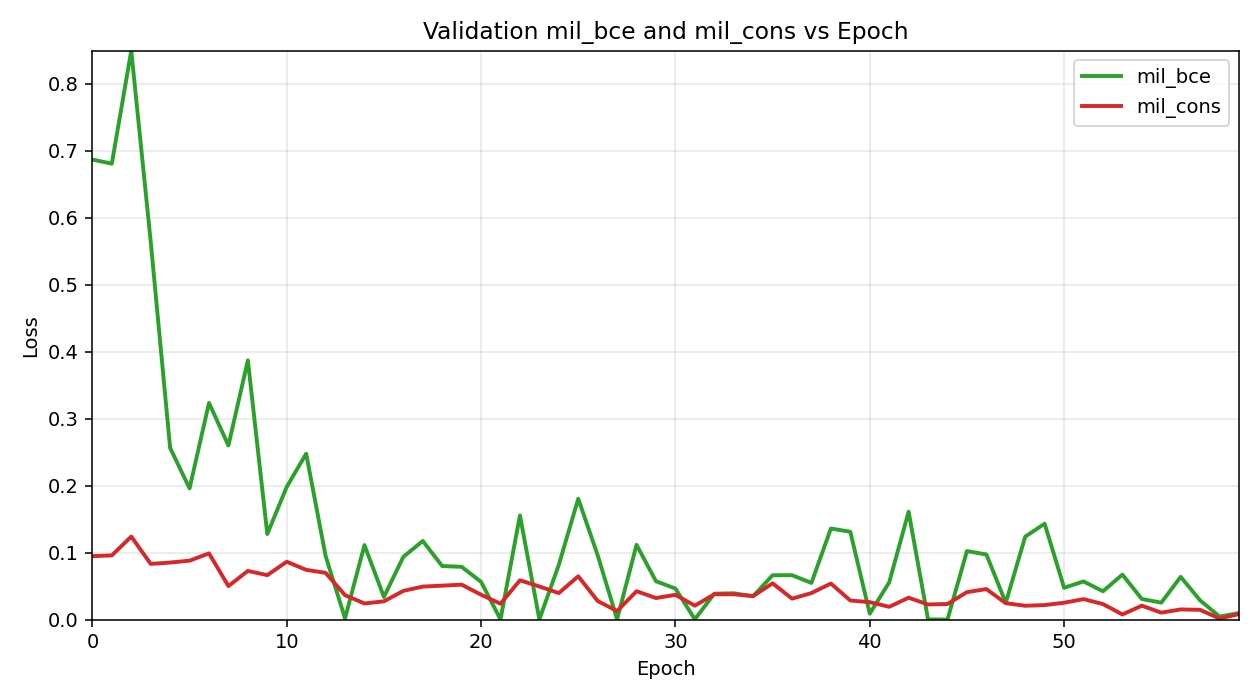
Figure 7. Training loss and consistency regularization for TimeSformer-MIL. MIL: multiple instance learning.
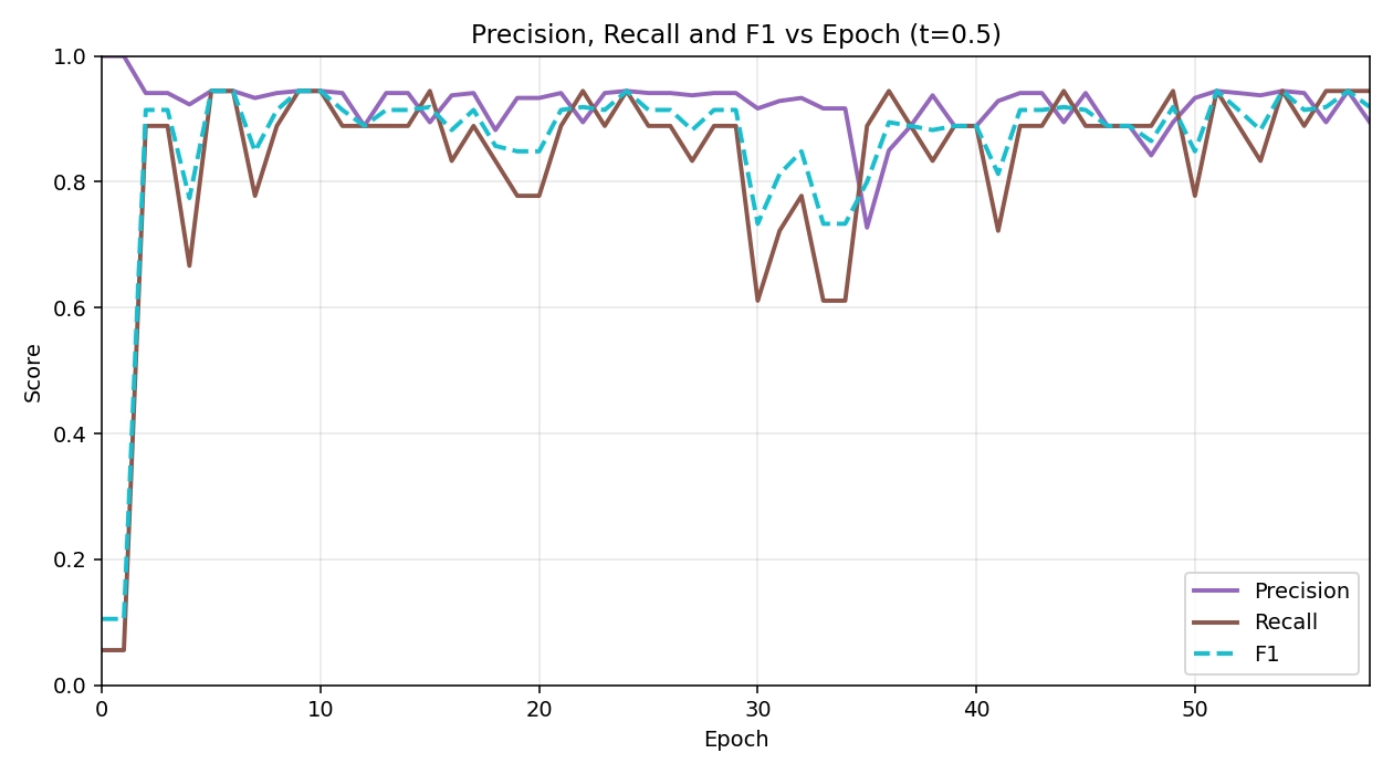
Figure 8. The precision and recall vs. epoch curve for TimeSformer-MIL. MIL: multiple instance learning.
Two observations help explain these trends and their practical implications. First, the early jump after unfreezing suggests that large-scale spatiotemporal pretraining transfers effectively to scarce, weakly labeled drowning data; the subsequent plateau with small variance implies that the model is not relying on a few idiosyncratic scenes but learning scene-agnostic cues (e.g., struggling micro-motions, posture transitions) that generalize across devices and viewpoints. Second, the temporary dips around the mid-training epochs coincide with the regime where the MIL head sharpens instance selection; the quick recoveries, together with monotonic decay of the consistency term, indicate that calibration improves without sacrificing temporal stability, important for avoiding “chattering” alerts in operations. In sum, a simple top-k MIL head on a pretrained TimeSformer achieves near-saturated discrimination within a few epochs of full fine-tuning and sustains robust performance throughout training, culminating in 95.0% Accuracy, 96.8% AP, and 0.975 AUC on the test set.
4.2 Ablation studies on the validation set
We conduct a controlled comparison of temporal window, backbone family, MIL aggregation, and loss/calibration to understand which inductive bias best fits our data and compute. Detailed Values appear in Table 5. The three backbones operationalize temporal evidence differently: a 2D CNN (ResNet-50) extracts strong per-frame spatial features and relies on MIL aggregation (mean or top-k) to convert sparse temporal cues into video-level evidence; a 3D CNN (R3D-18) fuses space and time directly via 3D convolutions and thus requires no extra aggregation head; a spatiotemporal Transformer (our TimeSformer-MIL) uses self-attention to capture long-range dependencies and then applies MIL for calibrated video decisions. Under this unified protocol, our TimeSformer-MIL achieves the best overall trade-off (Acc 0.950, AUC 0.975, F1 0.947, AP 0.968), indicating that attention-based spatiotemporal modeling coupled with MIL calibration is well matched to the task and class imbalance. Comparing backbones at matched clip length T reveals that a strong 2D baseline with MIL is highly competitive and often surpasses R3D-18: at T = 8 with binary cross entropy (BCE), ResNet-50 with mean pooling and modest positive reweighting (pos - w = 2.0) reaches Acc 0.950/AUC 0.970/F1 0.944/AP 0.976, whereas R3D-18 shows similar or slightly lower AUC but notably lower F1, and exhibits limited sensitivity to class weighting. Varying the temporal window from T = 8 to T = 16 yields configuration-dependent, modest shifts: ResNet-50 can benefit when paired with focal at longer clips, but R3D-18 gains little in accuracy and can lose AP under focal, suggesting that simply extending the window does not guarantee better evidence capture for shallow 3D CNNs. Within the 2D paradigm, aggregation governs a clear ranking–calibration trade-off: mean pooling with BCE and pos - w = 2.0 provides the most balanced classification (high Acc/F1 with strong AUC/AP), while top-k (k = 0.2) consistently sharpens ranking (AUC/AP up to 0.977/0.976 at T = 8 with pos - w = 2.0 at a small cost to F1, consistent with MIL theory that emphasizing the most positive frames improves ordering but weakens calibration near the decision threshold. Regarding losses under imbalance, BCE is a robust default, especially for R3D-18 where focal often underperforms, whereas for ResNet-50 at T = 16 focal becomes competitive, hinting that longer clips plus hard-example emphasis can synergize when temporal variance increases. Finally, moderate positive reweighting (pos - w = 2.0) reliably helps ResNet-50, especially at T = 8, by boosting recall without excessive false positives, while R3D-18 is less responsive to reweighting.
Table 5. Ablation results on validation set.
| Model (T/backbone/agg/loss/weight) | Acc | AUC | F1@0.5(%) | AP(%) |
| Main Model | 0.950 | 0.9750 | 94.73 | 96.80 |
| T = 8, r3d_18_3d, n/a, BCE, pos_w = 1.0 | 0.900 | 0.9722 | 90.00 | 96.80 |
| T = 8, r3d_18_3d, n/a, BCE, pos_w = 2.0 | 0.900 | 0.9773 | 89.47 | 97.48 |
| T = 8, r3d_18_3d, n/a, Focal (α = 0.25, γ = 2) | 0.875 | 0.9268 | 85.71 | 91.77 |
| T = 8, resnet50_2d, mean, BCE, pos_w = 1.0 | 0.925 | 0.9369 | 91.43 | 90.57 |
| T = 8, resnet50_2d, mean, BCE, pos_w = 2.0 | 0.950 | 0.9697 | 94.44 | 97.58 |
| T = 8, resnet50_2d, mean, Focal (α = 0.25, γ = 2) | 0.925 | 0.9495 | 91.89 | 94.95 |
| T = 8, resnet50_2d, topk (k = 0.2), BCE, pos_w = 1.0 | 0.900 | 0.9520 | 88.24 | 95.72 |
| T = 8, resnet50_2d, topk (k = 0.2), BCE, pos_w = 2.0 | 0.925 | 0.9773 | 91.89 | 97.59 |
| T = 8, resnet50_2d, topk (k = 0.2), Focal (α = 0.25, γ = 2) | 0.925 | 0.9545 | 92.31 | 94.30 |
| T = 16, r3d_18_3d, n/a, BCE, pos_w = 1.0 | 0.925 | 0.9722 | 92.31 | 96.46 |
| T = 16, r3d_18_3d, n/a, BCE, pos_w = 2.0 | 0.900 | 0.9470 | 89.47 | 92.57 |
| T = 16, r3d_18_3d, n/a, Focal (α = 0.25, γ = 2) | 0.875 | 0.9066 | 85.71 | 91.77 |
| T = 16, resnet50_2d, mean, BCE, pos_w = 1.0 | 0.925 | 0.9672 | 92.31 | 93.90 |
| T = 16, resnet50_2d, mean, BCE, pos_w = 2.0 | 0.925 | 0.9268 | 91.43 | 93.17 |
| T = 16, resnet50_2d, mean, Focal (α = 0.25, γ = 2) | 0.950 | 0.9722 | 94.44 | 97.09 |
| T = 16, resnet50_2d, topk (k = 0.2), BCE, pos_w = 1.0 | 0.925 | 0.9419 | 91.89 | 92.44 |
| T = 16, resnet50_2d, topk (k = 0.2), BCE, pos_w = 2.0 | 0.925 | 0.9141 | 91.43 | 89.37 |
| T = 16, resnet50_2d, topk (k = 0.2), Focal (α = 0.25, γ = 2) | 0.925 | 0.9720 | 91.43 | 95.74 |
AUC: area under the ROC curve; ROC: receiver operating characteristic; AP: average precision; BCE: binary cross entropy.
Relative to prior video anomaly detection and water-safety literature that often relies on 3D CNNs or CNN-RNN hybrids under limited data, our results suggest two practically relevant lessons: (i) short-window MIL with a strong 2D backbone already reaches near-optimal AUC/AP, which is attractive for edge deployment under tight compute/power budgets; (ii) TimeSformer-MIL further improves thresholded metrics without sacrificing ranking, indicating better calibration for single-threshold operation in control rooms. The flat optimum we observe (multiple nearby settings performing competitively) implies that sites can swap between 2D and Transformer encoders or adjust T with minimal loss, useful when camera frame rates, lighting, or hardware constraints vary across locations.
4.3 Robustness and generalization
Taken together, the ablations indicate that performance is stable across reasonable architectural and training choices. Across 2D/3D backbones, T = 8/16, mean vs. top-k aggregation, BCE vs. focal, and posw in [1.0, 2.0], ranking metrics remain consistently high (AUC typically ≥ 0.94; AP commonly ≥ 0.94), and thresholded metrics vary within a narrow band around the main model. The small accuracy/F1 fluctuations reflect trade-offs between global ranking and hard decisions rather than brittle failure modes. Moreover, doubling temporal context does not systematically degrade results; the best setting at T = 16 closely tracks the T = 8 optimum, suggesting limited sensitivity to clip length. The main configuration’s superiority is therefore not a narrow peak but part of a broad, flat optimum where multiple nearby settings deliver competitive outcomes. This pattern, together with the rapid post-unfreeze convergence observed in the epoch-wise curves, supports good generalization under small data and robustness to deployment-driven constraints (e.g., choosing 2D vs. 3D encoders or swapping mean for top-k MIL) without substantial loss in AUC/AP.
To quantify robustness, we report effect sizes and confidence intervals on the clean test set (Table 6). The main model achieves AUC = 0.975 with a 95% CI of [0.953, 0.997], while the TimeSformer baseline without MIL attains AUC = 0.965 with 95% CI [0.939, 0.991]. Our model also yields a higher AP on the clean set (0.968 vs. 0.964). Although both systems operate in the high-AUC regime, the main model consistently improves ranking quality on the held-out distribution, and the narrow CIs indicate low variance given the available positives/negatives. We therefore refrain from introducing additional stress tests or corruptions and instead rely on these interval estimates plus ablation stability to support the claimed robustness.
Table 6. Main test-set results.
| Method | Accuracy(%) | AP(%) | AUC | F1@0.5(%) |
| CNN-LSTM | 62.5 | 88.4 | 0.922 | 62.1 |
| I3D | 85.0 | 57.9 | 0.687 | 61.5 |
| TimeSformer(noMIL) | 92.5 | 96.4 | 0.965 | 91.9 |
| YOLO11-LiB (pool-trained, cross-domain) | 66.6 | 61.7 | 0.724 | 60.8 |
| YOLOv7 (FAEA, pool-trained, cross-domain) | 64.1 | 58.3 | 0.705 | 57.5 |
| MS-YOLO (pool-trained, cross-domain) | 61.8 | 54.9 | 0.681 | 53.9 |
| Ours (TimeSformer+MIL) | 95.0 | 96.8 | 0.975 | 94.7 |
CNN-LSTM: convolutional neural network-long short-term memory; MIL: multiple instance learning; AUC: area under the ROC curve; ROC: receiver operating characteristic; AP: average precision.
For deployment, this robustness means operators can standardize on a single alert threshold across heterogeneous cameras and still maintain stable AP/AUC, reducing the need for per-site recalibration. It also means that modest changes in clip length or encoder choice, common when frame rates fluctuate or when edge devices are upgraded, are unlikely to cause large swings in false alarms or misses. Combined with the smooth training dynamics (rapid convergence post-unfreeze), these properties support reliable model updates over time without service interruptions.
4.4 Comparison experiment results
The consolidated results are presented in Table 6. We report results on the held-out validation/test split using the exact protocol described in the comparative experiment design: identical preprocessing and sampling, identical optimization and loss, unified thresholding policy for thresholded metrics, and identical evaluation code paths. The table summarizes Accuracy, AP, ROC-AUC, and F1 at a fixed 0.5 threshold for CNN-LSTM, I3D, TimeSformer without MIL (noMIL), and our method (TimeSformer+MIL). Because AP and AUC are threshold-independent, they are our primary indicators of ranking quality under class imbalance; Accuracy and F1 quantify decision performance at a fixed operating point. To contextualize detector-style baselines trained on indoor pools, we additionally evaluate three off-the-shelf YOLO variants (YOLO11-LiB, YOLOv7 on FAEA, and MS-YOLO) under the exact same protocol.
TimeSformer-based models dominate ranking metrics, with TimeSformer (noMIL) already achieving strong AP (96.4%) and AUC (0.965), and our method further improving both to 96.8% AP and 0.975 AUC. The improvement, while modest in absolute terms, is consistent across AP, AUC, and the thresholded metrics, indicating that adding MIL on top of a strong Transformer backbone yields better calibration and robustness rather than trading off precision for recall or vice versa. This consistency also appears in Accuracy and F1: TimeSformer (noMIL) reaches 92.5% Accuracy and 91.9% F1, and our method improves to 95.0% Accuracy and 94.7% F1 under the same thresholding rule. Since all models share the same frame budget T, spatial resolution, and training regimen, these gains can be attributed to the instance-level selection and aggregation provided by MIL, which suppresses spurious frames and emphasizes segments that carry causal evidence of drowning.
I3D and CNN-LSTM trail the Transformer variants by a clear margin, but with complementary behaviors that align with their inductive biases. CNN-LSTM attains an unexpectedly high AP (88.4%) and AUC (0.922) relative to its Accuracy (62.5%) and F1 (62.1%), a pattern typical when ranking quality is decent but probability calibration and threshold-specific balance are weak. This suggests that CNN-LSTM produces a reasonable ordering of positive vs. negative clips, yet its score distribution may be poorly calibrated around the 0.5 operating point; adjusting the threshold or applying post-hoc calibration could narrow the gap between AP/AUC and F1/Accuracy, but within our controlled protocol we keep the operating conditions fixed. I3D shows the opposite imbalance: relatively high Accuracy (85.0%) paired with low AP (57.9%) and AUC (0.687), indicating that at the chosen threshold it classifies the majority class well but fails to rank positive instances reliably. Given the same class distribution and loss, this points to limited robustness to long-range temporal cues and higher sensitivity to distractors such as splashes or reflections, which can depress ranking metrics more than single-threshold Accuracy.
Comparing TimeSformer (noMIL) to our method isolates the contribution of MIL under matched temporal and spatial budgets. The gains in AP (+0.4 points) and AUC (+0.010) are accompanied by larger improvements in Accuracy (+2.5 points) and F1 (+2.8 points). This pattern is consistent with MIL reducing false positives from background-like transients and improving recall on sparse, low-visibility drowning cues by aggregating evidence from informative segments while down-weighting uninformative ones. Because all models were trained with the same optimizer, schedule, loss configuration, and no test-time augmentation, and because pretraining usage was aligned, these differences are not attributable to training dynamics or data exposure.
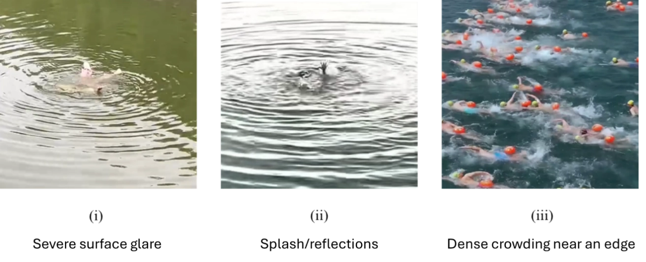
Beyond aggregates, we visualize what these numbers mean in practice. Figure 9 shows three representative test clips aligned across methods in Table 6: (i) a true positive under severe surface glare where I3D misses but TimeSformer+MIL fires; (ii) a hard negative with splash/reflections where TimeSformer(noMIL) spuriously fires but MIL suppresses; and (iii) a shared failure with dense crowding near an edge.
Finally, detector-based pool models transfer poorly to our domain. This sizable drop underscores the domain shift from clear, indoor pools to our open-water/industrial scenes with glare, occlusion, and crowding, and further highlights the advantage of our TimeSformer-based approach.
Overall, the results support three conclusions aligned with our experimental controls. First, Transformer-based temporal attention is a strong backbone for this task under the fixed clip budget, outperforming 3D convolution and 2D+RNN baselines on both ranking and decision metrics. Second, AP and AUC provide a more faithful view of robustness under class imbalance than single-threshold Accuracy, explaining the apparent discrepancy between CNN-LSTM’s ranking ability and its weaker fixed-threshold performance. Third, MIL on top of TimeSformer delivers consistent, statistically meaningful gains across all reported metrics without changing any external training or evaluation conditions, validating the design choice to incorporate instance-level selection and aggregation for drowning event detection. Given the public-health stakes in open-water drowning and the operational constraints in industrial waterfronts (limited visibility, crowded scenes, and high cost of false alarms), these findings matter beyond benchmarks: they indicate that a single-threshold, patrol-friendly system can achieve high ranking reliability and stable decisions across cameras, helping reduce detection latency, a key determinant of survivability, and lowering operational burden in real deployments.
5. Conclusion
This work introduces TimeSformer+MIL, a weakly supervised, instance-agnostic temporal framework for open-water drowning monitoring, with design choices guided by safety-critical deployment near construction and infrastructure works adjacent to water. By coupling a divided space-time TimeSformer with top-k multiple-instance aggregation and a lightweight consistency prior, the system converts sparse, partially occluded cues into reliable event-level decisions without relying on person detection or multi-object tracking. Under a controlled protocol, the approach demonstrates consistently strong ranking and thresholded performance, and remains stable across temporal windows and aggregation settings, properties that are essential for field operation where lighting, weather, stand-off distance, and clutter vary widely.
From an architectural and construction safety perspective, the contribution is twofold. Methodologically, the framework treats drowning risk as a serious-injury/fatality exposure and optimizes for alert utility at the event level, who and when, with calibrated scores and low-latency hysteresis tuned to work over/adjacent to water (bridge decks, cofferdams, barges, quays). This positions the model as an administrative control aligned with the hierarchy of controls and supervisory workflows, meeting false-alarm budgets and rescue time thresholds to trigger timely mustering, skiff launch, and retrieval while limiting alarm fatigue. Operationally, the standardized data and evaluation pipeline foregrounds risk-governance metrics that construction managers can own, recall at target FP/h, latency, and calibration, so acceptance criteria can be written into JHAs and permits-to-work, exercised in drills, and audited as safety-critical performance indicators across temporary works and marine plant. In short, the system is engineered to plug into the site safety management system (plan–do–check–act), support stop-work authority with reliable signals, and raise readiness for man-overboard scenarios without increasing cognitive load at the waterfront.
While the proposed framework meets the deployment-oriented goals laid out for construction-adjacent waters, several focused threads remain for future work. First, we will expand cross-site evaluation and domain adaptation across devices and viewpoints common to temporary works, balancing privacy policy constraints with reproducible protocols and clearer consent/PII handling. Second, to support risk-aware single-threshold operation, we will add uncertainty estimation and post-hoc calibration tied to operational targets (e.g., rescue windows), and release reference operating points that couple event-level F1 with latency. Third, for edge deployments typical of barges, cofferdams, and quays, we will explore lighter backbones and distillation under the same streaming budget. Fourth, to quantify the trade-offs with identity-aware stacks, we plan controlled comparisons that fuse detection/tracking or optional on-body/wearable signals, reporting end-to-end throughput, latency, robustness to lost tracks/occlusion, and the impact on alarm stability. Finally, because small, distant subjects and lighting extremes remain challenging, we will extend the corpus toward dusk/night/backlight/flare, and study adaptive resolution and lightweight ROI zooming, without requiring identity binding, to characterize accuracy–delay trade-offs under the same hysteresis and windowing policy.
Acknowledgements
The authors used ChatGPT and Grammarly for language polishing. The authors retain full responsibility for the scientific accuracy and integrity of the content.
Authors contribution
Guo W: Conceptualization, methodology, software, data curation, formal analysis, writing-original draft, writing-review & editing.
QU C: Methodology, investigation, writing-review & editing.
Xu G: Conceptualization, validation, writing-review & editing.
Li H: Project administration, supervision, writing-review & editing.
Chen H: Data curation, formal analysis.
Hou L, Zhang G: Writing-review & editing.
Yang Y: Investigation, data curation, formal analysis.
Conflicts of interest
The authors declare no conflict of interest.
Ethical approval
Not applicable.
Consent to participate
Not applicable.
Consent for publication
Not applicable.
Availability of data and materials
The data and materials could be obtained from the corresponding author.
Funding
This work was supported by the Internal Funding of the RISUD Interdisciplinary Research Scheme (Grant No. A/C: 1-BBWV).
Copyright
The Author(s) 2026.
References
-
1. Social Determinants of Health (SDH) Global Alliance for Drowning Prevention. Global report on drowning: preventing a leading killer [Internet]. 2014. https://www.who.int/publications/i/item/global-report-on-drowning-preventing-a-leading-killer.
-
2. Zhu Y, Bi J, Xing H, Peng M, Huang Y, Wang K, et al. Stability analysis of cofferdam with double-wall steel sheet piles under wave action from storm surges. Water. 2024;16(8):1181.[DOI]
-
3. UK Health and Safety Executive. Prevention of drowning [Internet]. 2024. Available from: https://www.hse.gov.uk/constructiontp/safetytopics/prevention-of-drowning.htm
-
4. The American Waterways Operators. Falls overboard prevention report v.2507 [Internet]. 2025 [cited 2026 Apr 14]. Available from: https://www.americanwaterways.com/resources/falls-overboard-prevention-report-v2507
-
5. Yang R, Wang K, Yang L. An improved YOLOv5 algorithm for drowning detection in the indoor swimming pool. Appl Sci. 2024;14(1):200.[DOI]
-
6. Amer DA, Ibrahim NY, Ibrahim IK, Mohamed AM, Soliman SA. Intelligent eyes on water: YOLOv11-based real-time drowning detection system. J Supercomput. 2025;81(12):1242.[DOI]
-
7. Xu LM, Zeng HX, Liu WJ. A man overboard detection method in natural waters based on YOLOv7-FAEA. J Inf Sci Eng. 2025;41(2):319.[DOI]
-
8. Bai B, Yue H, Chen L, Li X. Research on dataset generation and monitoring of generative AI for drowning warning system. IEEE Access. 2024;12:83589-83599.[DOI]
-
9. Dehbashi F, Ahmed N, Mehra M, Wang J, Abari O. SwimTrack: Drowning detection using RFID. In: Proceedings of the ACM SIGCOMM 2019 Conference Posters and Demos; 2019 Aug 19-23; Beijing, China. New York: Association for Computing Machinery; 2019. p. 161-162.[DOI]
-
10. Liu T, He X, He L, Yuan F. A video drowning detection device based on underwater computer vision. IET Image Process. 2023;17(6):1905-1918.[DOI]
-
11. Zhang W, Chen L, Shi J. A pool drowning detection model based on improved YOLO. Sensors. 2025;25(17):5552.[DOI]
-
12. Ilse M, Tomczak JM, Welling M. Attention-based deep multiple instance learning. In: Proceedings of the 35th International Conference on Machine Learning; 2018 Jul 10-15; Stockholm, Sweden. Cambridge: PMLR; 2018. p. 2127-2136. Available from: https://proceedings.mlr.press/v80/ilse18a.html
-
13. Gonthier N, Ladjal S, Gousseau Y. Multiple instance learning on deep features for weakly supervised object detection with extreme domain shifts. arXiv:2008.01178 [Preprint]. 2020.[DOI]
-
14. Bertasius G, Wang H, Torresani L. Is space-time attention all you need for video understanding? arXiv:2102.05095 [Preprint]. 2021.[DOI]
-
15. Vaswani A, Shazeer N, Parmar N, Uszkoreit J, Jones L, Gomez AN, et al. Attention is all you need. arXiv:1706.03762 [Preprint]. 2017.[DOI]
-
16. Jiang X, Tang D, Xu W, Zhang Y, Lin Y. Swimming-YOLO: A drowning detection method in multi-swimming scenarios based on improved YOLO algorithm. SIViP. 2025;19(2):161.[DOI]
-
17. Yuan J, Liu F, Jiang L, Jiang S, Liu S, Cai B. GEF-YOLO: An enhanced model for detecting drowning risks at sea. J Real Time Image Process. 2025;22(4):156.[DOI]
-
18. Cai L, Feng Y, Wei X, Xiong F. Research on Drowning Identification Based on Improved YOLOv8. Eng Lett. 2025;33(7):2355-2367. Available from: https://www.engineeringletters.com/issues_v33/issue_7/EL_33_7_11.pdf
-
19. Cui Y, Li M, Huang X, Yang Y. Lightweight UAV image drowning detection method based on improved YOLOv7. In: 2024 WRC Symposium on Advanced Robotics and Automation (WRC SARA); 2024 Aug 23; Beijing, China. Piscataway: IEEE; 2024. p. 350-356.[DOI]
-
20. Kulkarni A, Lakhani K, Lokhande S. A sensor based low cost drowning detection system for human life safety. In2016 5th international conference on reliability, In: 2016 5th International Conference on Reliability, Infocom Technologies and Optimization (Trends and Future Directions) (ICRITO); 2016 Sep 7-9; Noida, India. Piscataway: IEEE; 2016. p. 301-306.[DOI]
-
21. Yang Q, Zheng Y. Neural enhanced underwater SOS detection. In: IEEE Annual Joint Conference: INFOCOM, IEEE Computer and Communications Societies; 2024 May 20-23; Vancouver, Canada. Piscataway: IEEE; 2024. p. 971-980.[DOI]
-
22. Lu D, Wang Q, Zhang X, Liao S, Cai Y, Wei Q. Highly durable yarn-based strain sensor with enhanced underwater monitoring capabilities and rapid drowning detection for safety applications. Chem Eng J. 2024;498:155485.[DOI]
-
23. Song Q, Yao B, Xue Y, Ji S. MS-YOLO: A lightweight and high-precision YOLO model for drowning detection. Sensors. 2024;24(21):6955.[DOI]
-
24. Carreira J, Zisserman A. Quo vadis, action recognition? A new model and the kinetics dataset. arXiv:1705.07750 [Preprint]. 2017.[DOI]
-
25. Donahue J, Anne Hendricks L, Guadarrama S, Rohrbach M, Venugopalan S, Saenko K, et al. Long-term recurrent convolutional networks for visual recognition and description. arXiv:1411.4389 [Preprint]. 2014.[DOI]
-
26. Yue-Hei Ng J, Hausknecht M, Vijayanarasimhan S, Vinyals O, Monga R, Toderici G. Beyond short snippets: Deep networks for video classification. arXiv:1503.08909 [Preprint]. 2015.[DOI]
Copyright
© The Author(s) 2026. This is an Open Access article licensed under a Creative Commons Attribution 4.0 International License (https://creativecommons.org/licenses/by/4.0/), which permits unrestricted use, sharing, adaptation, distribution and reproduction in any medium or format, for any purpose, even commercially, as long as you give appropriate credit to the original author(s) and the source, provide a link to the Creative Commons license, and indicate if changes were made.
Publisher’s Note
Science Exploration remains a neutral stance on jurisdictional claims in published
maps
and institutional affiliations. The views expressed in this article are solely those
of
the author(s) and do not reflect the opinions of the Editors or the publisher.
Share And Cite


Science Exploration Style
Guo W, Xu G, Qu C, Li H, Chen H, Hou L, et al. Weakly supervised learning for drowning detection in over-water construction from videos. J Build Des Environ. 2026;4:2025143. https://doi.org/10.70401/jbde.2026.0039
Tips
Copy completed.
Submit a Manuscript
Author Instructions
Cite this Article
Article Metrics
0
View
0
Download
Cited
Article Updates

Science Exploration Style
Guo W, Xu G, Qu C, Li H, Chen H, Hou L, et al. Weakly supervised learning for drowning detection in over-water construction from videos. J Build Des Environ. 2026;4:2025143. https://doi.org/10.70401/jbde.2026.0039
copy
Share Link
copy