Life cycle techno-economic analysis and optimization framework of hybrid deep ground source heat pump system for low carbon buildings

*Correspondence to:
Yongqiang Luo, School of Environmental Science and Engineering, Huazhong University of Science and Technology, Wuhan 430074, Hubei, China.
E-mail: yqluo@hust.edu.cn
J Build Des Environ. 2026;4:202621. 10.70401/jbde.2026.0041
Received: May 05, 2026Accepted: July 17, 2026Published: July 17, 2026
Abstract
This study develops a life-cycle techno-economic analysis and optimization framework for hybrid deep ground source heat pump (GSHP) systems, addressing the limitations of existing evaluations that often neglect subsurface thermal attenuation and rely on simplified heat transfer models. A coupled heat transfer model is established by combining the finite difference method for the borehole interior with the segmented finite line-source model for the surrounding ground, enabling long-term simulation of fluid and ground temperature evolution. The energy model is integrated with a life-cycle economic evaluation to calculate net present value, levelized cost of heating/cooling, payback period (PP), and internal rate of return. A Bayesian optimization algorithm is further employed to identify optimal system configurations under multiple objectives. The framework is applied to a hybrid geothermal system in Xi’an, China, incorporating mid-deep boreholes with auxiliary air-source heat pumps or gas boilers. Results show that long-term thermal attenuation significantly affects economic performance, with a 2 °C increase in fluid temperature extending the PP by approximately 0.3 years. User-side load uncertainty also has a substantial impact, as a 10% deviation from the design load can shift the optimal PP by about 2 years. Sensitivity analysis identifies the GSHP installed capacity ratio and borehole number as the most influential parameters. Compared with pure geothermal systems, the hybrid geothermal–gas boiler configuration achieves the shortest PP, demonstrating the framework’s effectiveness for robust low-carbon system design.
Keywords
Hybrid geothermal system, space heating, optimization, life cycle analysis
1. Introduction
Geothermal energy is a renewable resource capable of providing consistent baseload power and overcoming the limitations of intermittent sources like wind and solar[1]. Geothermal Systems represent a transformative technology that can unlock vast thermal resources from deep rock formations. This substantially expands geothermal geographical applicability, positioning it as a vital element in diversified decarbonization strategies[2]. When integrated into 100% renewable energy systems, enhanced geothermal systems (EGS) can reduce system costs by approximately 60% compared to business-as-usual scenarios while decreasing land requirements and storage needs[1]. Life cycle assessments (LCA) reveal that the carbon intensity of geothermal heating is significantly lower than that of conventional fossil fuel systems[3]. For instance, a cradle-to-grave assessment showed that repurposing abandoned oil and gas wells for district heating can reduce the global warming potential by up to 24% over 30 years compared to natural gas-fired systems[4]. Furthermore, geothermal direct-use applications can provide industrial process heat without combustion, thereby eliminating both CO2 and harmful air pollutants from manufacturing. The development of this sector is strongly influenced by policy measures. One study indicates that heat premiums are the most cost-efficient policy instrument for reducing project abandonment rates, highlighting the need for supportive regulatory frameworks[5].
The optimization and design of geothermal energy systems constitute a critical research frontier that directly determines the technical feasibility, economic viability, and environmental sustainability of geothermal power generation. As the global energy transition accelerates, the systematic optimization of geothermal system configurations, working fluid selection, and operational parameters has become indispensable for unlocking the full potential of this baseload renewable resource.
A central focus in contemporary geothermal research is the multi-objective optimization of thermodynamic cycles, which enables the simultaneous balancing of competing performance criteria such as net power output, investment cost, and carbon emissions. Recent studies have established comprehensive tri-objective frameworks incorporating thermo-economic and environmental indicators to guide critical decisions in system configuration[6]. The optimization of combined heat and power configurations represents another vital dimension of geothermal system design. Advanced thermodynamic comparisons between direct supercritical carbon dioxide concepts and indirect brine-organic Rankine cycle systems have demonstrated that heat carrier selection profoundly influences system responsiveness to varying heat demand, with sCO2 configurations exhibiting substantially higher sensitivity while achieving an average exergetic efficiency approaching 72.6%, compared to approximately 40% for brine-based alternatives[7]. Addressing operational uncertainties and subsurface complexity constitutes a third critical aspect of geothermal optimization research. Robust optimization frameworks integrating genetic algorithms with geothermal plant simulators have been developed to enhance operational resilience under uncertain heating demands[8]. For multi-generation systems producing electricity, cooling, and hydrogen, genetic algorithm-based optimization has identified optimal operating configurations with exergy efficiencies of 38.96%[9]. Additionally, machine-learning-accelerated multi-objective optimization frameworks have emerged as transformative tools for enabling efficient management of fractured geothermal systems, achieving remarkable simulation speed-ups of one to two orders of magnitude compared to traditional evolutionary methods[10]. These advances are complemented by quantum machine learning-driven surrogate modeling approaches capable of transforming computationally intractable optimization problems into rapid calculations while maintaining prediction accuracy comparable to full-physics models.
LCA has emerged as an indispensable methodological framework for comprehensively evaluating the environmental sustainability of geothermal energy systems, enabling rigorous quantification of impacts across all stages from resource extraction and plant construction to operation and final decommissioning. At the plant level, detailed LCA case studies illuminate critical insights into the distribution of environmental burden across the facility life cycle. An LCA of the Hellisheidi geothermal combined heat and power plant in Iceland, applying life cycle impact assessment with CML-IA baseline and Cumulative Energy Demand methods, found that the construction phase, particularly drilling and casing of geothermal wells, dominates most environmental impact categories[11]. The environmental benefits of geothermal systems are further substantiated through comparative and hybrid LCA applications. A cradle-to-grave prospective LCA comparing a geothermal district heating system repurposing inactive oil and gas wells with conventional natural gas-fired heating demonstrated a reduction in global warming potential of up to 24% over a 30-year operational period, with cumulative greenhouse gas reductions increasing over time as a function of future renewable resource penetration[4]. This highlights the dual environmental advantage of repurposing existing fossil fuel infrastructure for clean energy production. For shallow geothermal applications, an LCA of ground source heat pump (GSHP) systems compared to air source heat pumps revealed lower long-term environmental impacts for GSHP configurations, primarily because the ground’s constant year-round temperature improves operational efficiency[12]. The integration of geothermal energy with other renewable sources has also been examined through LCA. For hybrid geothermal-biomass combined power cycles, detailed exergetic, environmental, and economic appraisals demonstrated that optimized hybridization modes can achieve CO2 emission reductions of up to 22.5% compared to less integrated configurations[13]. Furthermore, a comprehensive review of life cycle sustainability and circular economy perspectives found that geothermal power plants can be economically competitive with solar photovoltaic, hydro, and wind energy sources when considering life cycle costing[14]. While prior studies have applied environmental LCA, the present study focuses on life-cycle techno-economic performance and operational carbon-emission comparison.
In addition, Frick et al.[15] conducted one of the most representative LCAs of geothermal binary power plants using enhanced low-temperature reservoirs, showing that the environmental performance of geothermal electricity is strongly affected by site-specific geological conditions, drilling depth, plant configuration, and auxiliary energy demand. Lacirignola and Blanc[16] further extended LCA to EGS by comparing multiple practical design options, indicating that reservoir stimulation, well construction, and induced-seismicity-related design choices are important factors affecting life-cycle environmental burdens. From an optimization perspective, Gerber and Maréchal[17] proposed an environomic framework for identifying optimal geothermal energy conversion configurations, demonstrating that environmental and economic objectives should be considered simultaneously in the design of future EGS projects. More recent studies have shifted attention to regional and application-specific assessments. Wang et al.[18] compared different geothermal power generation technologies in China and found that environmental impacts vary significantly among flash, binary, and EGS due to differences in resource conditions, system configuration, and drilling requirements. For geothermal heating applications, Xia et al.[19] developed a multi-objective optimization method for geothermal heating systems based on thermal-economic and environmental impact evaluation, providing a more systematic approach for selecting sustainable system parameters. Overall, the literature shows that geothermal energy generally has considerable low-carbon potential, but its life-cycle performance is highly dependent on geological conditions, drilling and construction processes, operational electricity consumption, system configuration, and optimization strategy. Therefore, future geothermal system design should integrate LCA, techno-economic analysis, and multi-objective optimization to achieve a balanced improvement in environmental sustainability, energy efficiency, and economic feasibility.
Although there are many studies on optimization and life cycle analysis[20] of geothermal system, few have integrated detailed heat-transfer models into system-level evaluations. Most existing studies rely on simplified evaluation models, such as constant system efficiency assumptions or overly simplified empirical formulas. For example, Dong et al.[21] estimated the heat extraction rate of a deep borehole heat exchanger using a steady-state formula. Because standalone geothermal systems can rarely meet the full heating and cooling demand, integration with auxiliary heating or cooling sources is a practical solution; however, few studies have provided a comprehensive evaluation and optimization procedure for such hybrid systems. More importantly, few studies have considered performance degradation in life-cycle analysis, which is one of the major factors distinguishing geothermal system optimization from that of other renewable energy systems. Heat extraction from geothermal boreholes gradually declines during annual operation, meaning that life-cycle analysis cannot simply repeat the first-year operating cost over the entire project lifetime. In addition, the effects of variable occupancy rate, borehole structure, and economic parameters on system optimization have also been insufficiently explored.
Based on the identified research gaps, this study proposes a comprehensive life-cycle techno-economic analysis and optimization framework for hybrid geothermal systems. The main contributions are as follows: (1) an analytical borehole heat-exchanger model is integrated with an economic model to evaluate long-term operating costs more accurately, rather than relying on simplified operating-cost estimates that neglect performance degradation; (2) a Bayesian optimization algorithm (BOA) is coupled with the economic model to achieve global optimization of hybrid geothermal systems with fewer iterations; and (3) detailed optimization analyses of deep geothermal systems are conducted to investigate the effects of multiple influencing factors and compare the optimization results of different hybrid geothermal configurations.
2. Methodology
2.1 Overview of system and method
2.1.1 Hybrid geothermal system
This study focuses on a hybrid heating and cooling system in which geothermal energy serves as the primary source, supplemented by other heating and cooling sources[22]. On the demand side, both heating and cooling loads are dynamic and typically peak in mid-winter and mid-summer. Designing a GSHP system based solely on the maximum heating or cooling load would result in excessively high initial investment, as it would require a large number of boreholes. In general, peak loads occur far less frequently than typical loads. Therefore, in practical engineering applications, a more commonly adopted solution is a hybrid geothermal heating and cooling system, in which geothermal energy provides the base load, while other heating and cooling sources are used for peak shaving. The GSHP operates as the primary energy source, supplemented by auxiliary systems depending on actual conditions. For cooling, options include standalone chillers or heat pumps combined with cooling towers. For heating, cost-effective, fast-response systems such as gas-fired or electric boilers are often employed to handle peak demands.
The geothermal heating and cooling system consists of a borehole heat-exchange system, a plant room equipped with heating and cooling equipment, and a terminal user system. As shown in Figure 1, the user side may require heating, cooling, or both from an overall perspective; however, the calculations assume that heating and cooling are not required simultaneously. For heating, medium-deep or shallow geothermal energy serves as the primary source, with auxiliary heat sources such as gas-fired or electric boilers and air-source heat pumps (ASHP). For cooling, shallow ground-source heat pumps are adopted as the main source and are supplemented by auxiliary systems such as heat pump units combined with cooling towers, similar to conventional chillers, or ASHP.
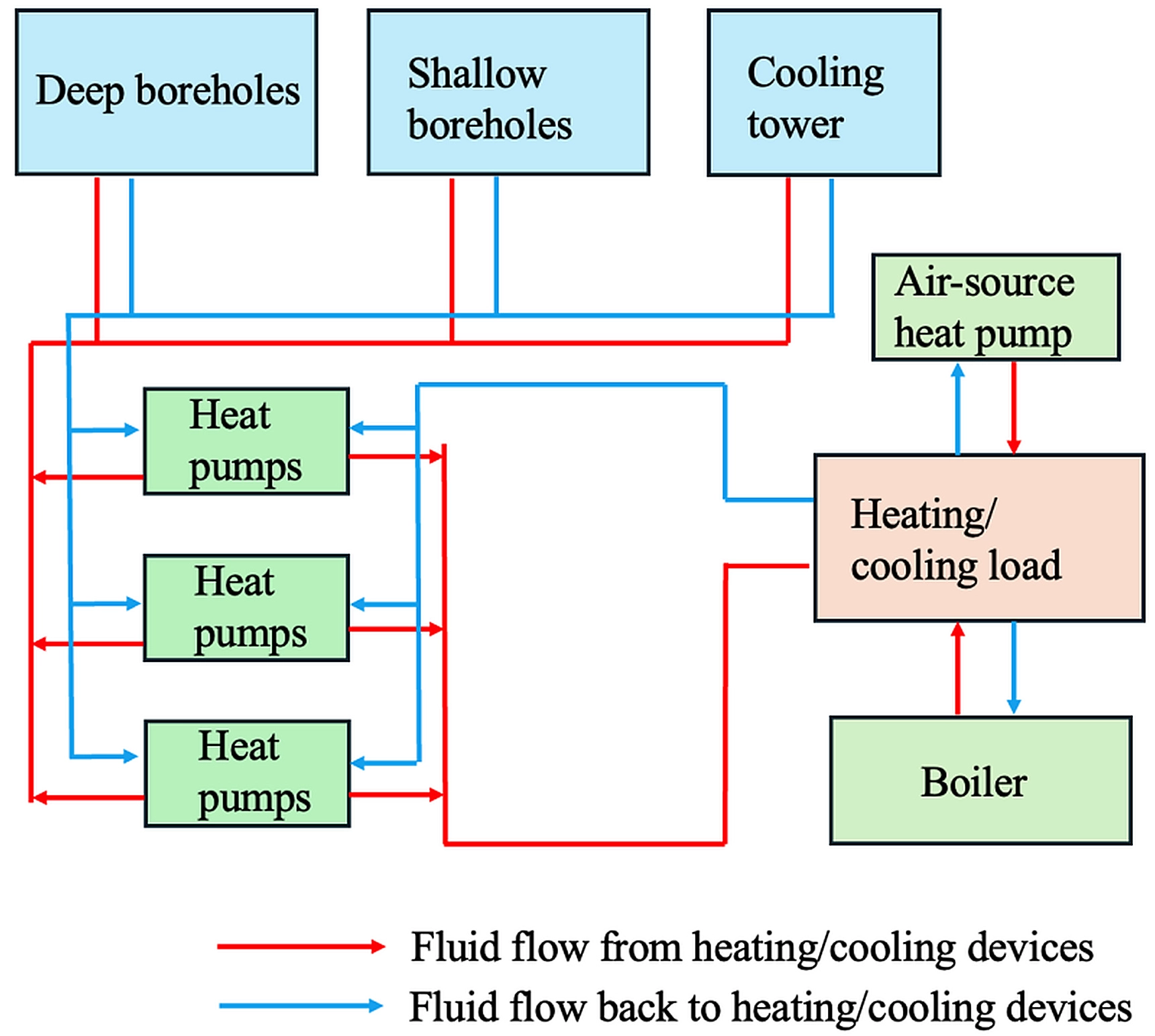
Figure 1. Schematic diagram of a hybrid geothermal and auxiliary heating and cooling system.
In the subsequent analysis, the heat transfer model of the borehole heat exchanger is used. First, the ratio of heating supply (RHS) of the borehole system is calculated under the constraint of the user-side load. When RHS is less than 1, auxiliary heating or cooling sources are employed to make up the deficit. In this way, the energy consumption of all equipment can be evaluated while ensuring that user-side demands are met. Based on the resulting energy consumption, further analyses of operating costs and environmental benefits can be carried out.
2.1.2 Method overview
Figure 2 illustrates the overall framework for the life-cycle techno-economic analysis of the medium–deep geothermal system, which mainly consists of four components: investment, operation cost, economic index, and integrated computation.
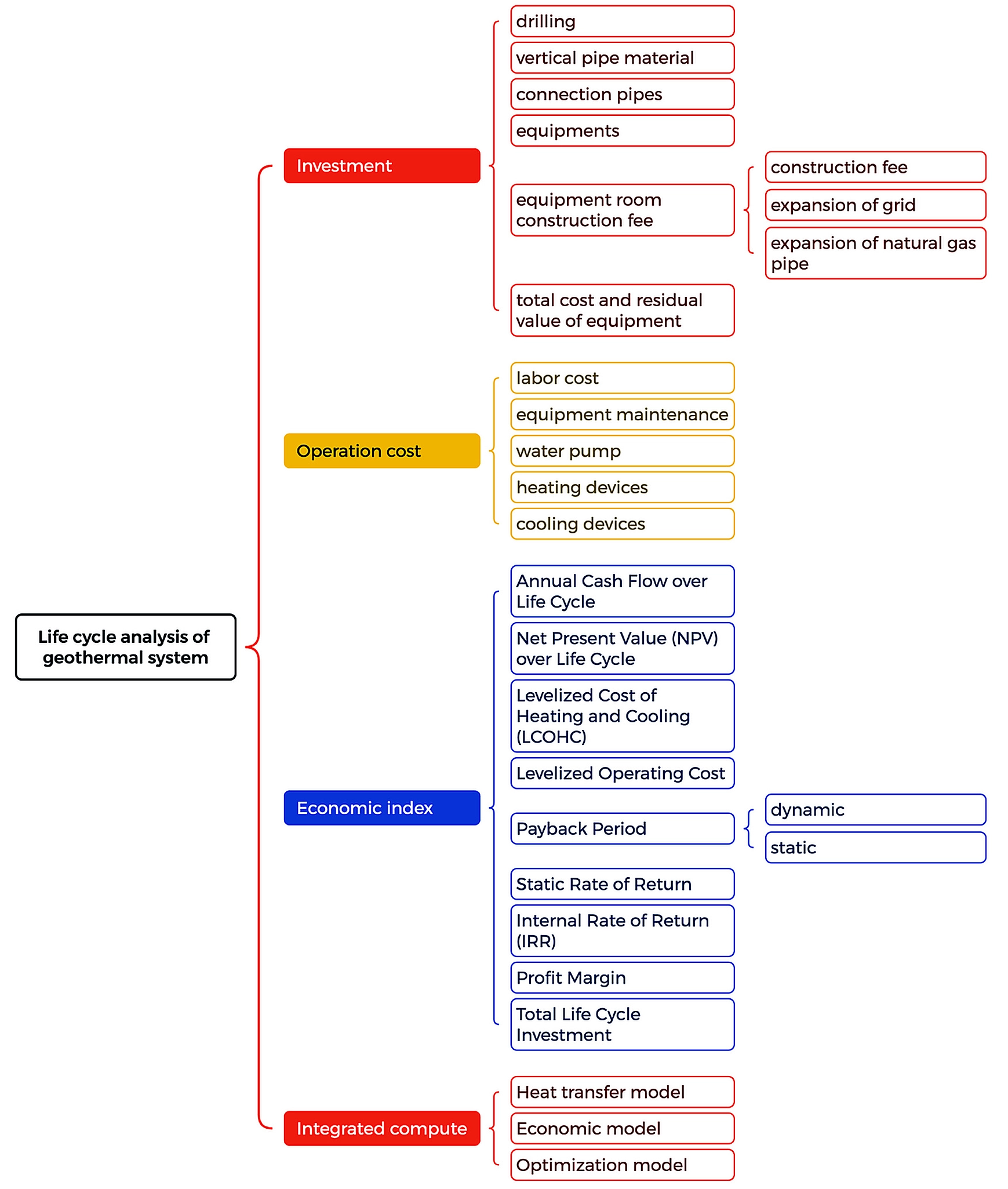
Figure 2. Life cycle techno-economic analysis framework of geothermal system.
First, in terms of investment, the system includes expenses for drilling, vertical pipe material, connection pipes, and equipment as part of the basic infrastructure. It also covers the construction cost of the equipment room and related supporting expenditures, such as power grid expansion and natural gas pipe extension. In addition, the total cost of equipment and its residual value are comprehensively taken into account.
Second, the operating cost mainly includes labor, equipment maintenance, and the energy-consumption costs of water pumps, heating devices, and cooling devices. These factors jointly determine the long-term operational and economic performance of the system.
In the economic index section, the figure presents several key indicators, including the annual cash flow over the full life cycle, net present value (NPV), levelized cost of heating and cooling, levelized operating cost, payback period (PP) (both dynamic and static), internal rate of return (IRR), and profit margin. These indicators are used to assess the economic feasibility and investment return of the system from multiple perspectives. When conducting system optimization, the loop takes economic indexes calculation in Figure 2 in each round and updates system parameters to meet the optimization objective.
2.2 Energy model
2.2.1 Model architecture
Figure 3 illustrates the complete solution procedure of the coupled heat transfer numerical model for borehole heat exchangers. The model adopts a hierarchical framework of Inputs–Main body–Output. The input module covers three categories of basic data: initial conditions, user side loads, and system and model parameters.
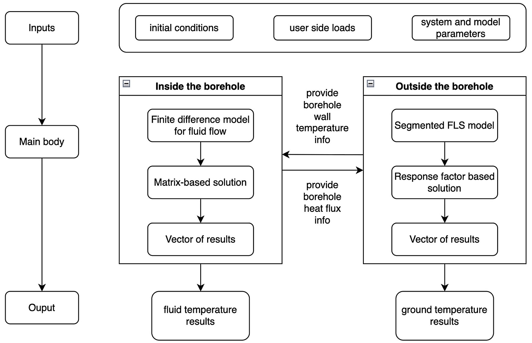
Figure 3. Borehole internal-external coupled heat transfer calculation framework.
The main calculation body consists of two bidirectionally coupled subsystems: the internal borehole subsystem and the external ground subsystem. The internal subsystem establishes a finite-difference model for fluid flow, solves the resulting matrix equation to obtain the result vector, and outputs the fluid-temperature results. Meanwhile, it provides borehole heat-flux information to the external subsystem. The external subsystem adopts a segmented finite line-source (FLS) model[23-25], uses a response-factor-based solution to obtain the result vector, and outputs the ground-temperature results. Meanwhile, it provides borehole-wall-temperature information to the internal subsystem.
The two sub-systems realize coupled iterative calculation via bidirectional boundary information transmission, which fully completes the fluid-stratum coupled heat transfer simulation of the borehole system. This finally outputs two core results: fluid temperature and ground temperature.
2.2.2 Heat transfer inside the borehole
As shown in Figure 4, the operation mode of the concentric coaxial borehole heat exchanger is illustrated below. Medium-deep borehole heat exchangers generally bear most heating loads, thus adopting the outer-in & inner-out operation mode, i.e., fluid flows into the outer pipe and out of the inner pipe. For shallow borehole heat exchangers, the same outer-in & inner-out mode is adopted during the heating season, whereas the inner-in & outer-out mode is applied during the cooling season.
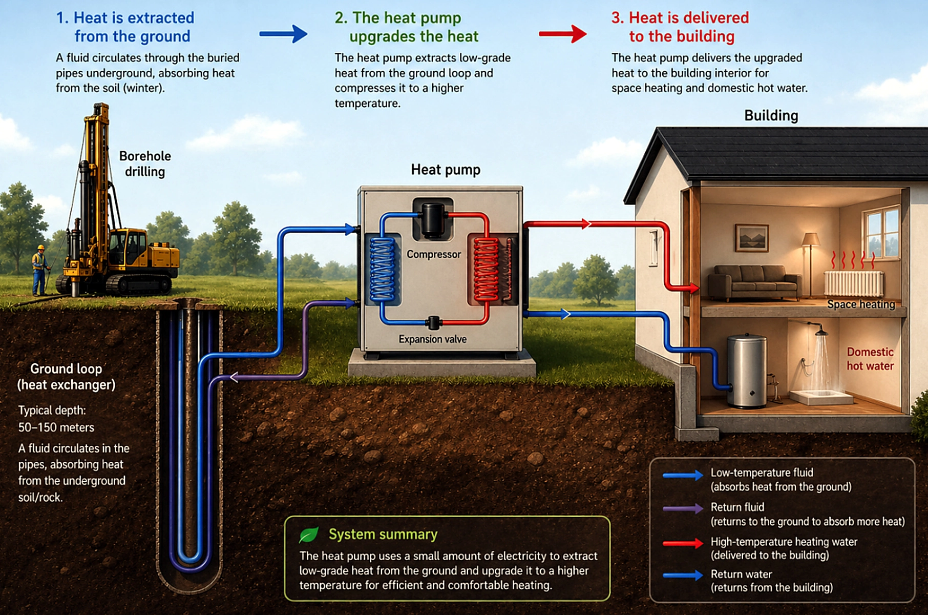
Figure 4. Schematic diagram of borehole heat exchanger, heat pump and buildings.
In this study, a coaxial borehole heat exchanger is selected, and its operation follows the outer-in & inner-out fluid flow pattern. The heat transfer in the borehole heat exchanger is mainly divided into two components: convective heat transfer of fluid inside the pipe and heat conduction outside the pipe. At the interface between the two components, both temperature and heat flux are consistent and equal. Considering practical engineering conditions, the model is simplified based on a series of assumptions as follows:
(a) Groundwater seepage is neglected in the external heat conduction around the borehole.
(b) The initial ground temperature is defined according to the geothermal gradient.
(c) The surface temperature is time-invariant and is set as a constant value.
(d) All thermophysical parameters involved in the model are assumed to be constant.
For the convective heat transfer of fluid inside the pipe, calculations are conducted via the Finite Difference Method and energy equations[24]. Equations (1) and (2) are derived from the energy equations. In these equations, C1 and C2 represent the per-unit-length thermal capacity of the outer pipe system (including pipe material, fluid and backfill material) and the inner pipe system (including pipe material and fluid), respectively, and their calculation methods are specified in Equations (3) and (4). R1 and R2 denote the thermal resistance between the outer pipe fluid and borehole wall, and that between inner and outer pipe fluids (W·K)/m, respectively, whose calculation formulas are given by Equations (5) and (6).
Where tb, tf1 and tf2 represent the temperatures of the borehole wall, outer pipe fluid and inner pipe fluid, respectively, in °C; M denotes the fluid mass flow rate inside the pipe, in kg/s; cf, c1, c2 and cg are the specific heat capacities of the fluid, outer pipe, inner pipe and grout, respectively, in J/(kg·°C); ρf, ρ1, ρ2 and ρg are the densities of the fluid, outer pipe, inner pipe and grout, respectively, in kg/m3; kp1, kp2 and kg are the thermal conductivities of the outer pipe, inner pipe and grout, respectively, in W/(m·K); h1 and h2 are the convective heat transfer coefficients of the annular channel and inner pipe, respectively, in W/(m2*K); db, d1o, d1i, d2o and d2i represent the borehole diameter, outer diameter and inner diameter of the outer pipe, as well as the outer diameter and inner diameter of the inner pipe, respectively, in m.
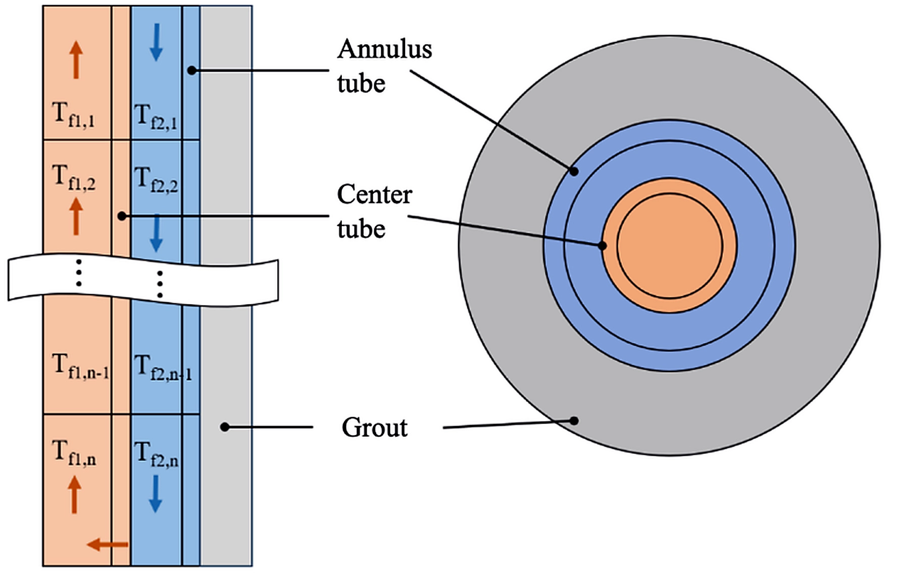
As shown in Figure 5, discretization is conducted for Equations (1) and (2) respectively, resulting in Equations (7) and (8). The superscript k represents the current time step, and superscript k + 1 denotes the next time step; n means that n spatial nodes are uniformly arranged along the depth direction inside the pipe. In addition, two boundary conditions are applied: constant inlet temperature (Tf1,1 = Tin) and identical fluid temperature at the bottom of the inner and outer pipes (Tf1,n = Tf2,n). On this basis, the fluid temperature at different moments can be solved. Specifically, this system of equations is converted into the form of Equation (9) by matrix operation.
2.2.3 Heat transfer outside the borehole
For heat conduction outside the borehole, the segmented FLS model is adopted for calculation. The temperature at each point can be regarded as the superposition of initial temperature and excess temperature generated by the heat source.
By discretizing the heat source into segments, the excess temperature at each position is obtained as shown in Equation (9)[25]. In subsequent calculations, to avoid redundant computation, all terms except heat flux in Equation (9) are rewritten into the corresponding coefficient matrix forms, as shown in Equation (10). Since the parameters in the coefficient matrix are independent of heat flux, the required coefficient matrix can be pre-calculated and stored for repeated calculations.
Where θ(r,z,τ) is the excess temperature at radius r (m) and depth z (m) after time duration τ (s), in °C; q represents heat flux, in W; Δτ is the time step, in s; k denotes thermal conductivity, in W/(m.K); and a is thermal diffusivity, in m2/s.
2.2.4 Energy model verification
The energy model is vital to provide thermal performance and subsequent operational costs of geothermal system. The model verification is conducted by monitoring data from a real engineering project in Xi’an, China. This is a 5 × 1 deep bore-field in line shape. The flow rate varies between 100-120 m3/h, and the system parameters are provided in the literature[26]. A comparison between simulated and measured outlet temperatures is presented in Figure 6. It is found that the energy model of geothermal system can accurately predict borehole temperature with an averaged error of 3.7%.
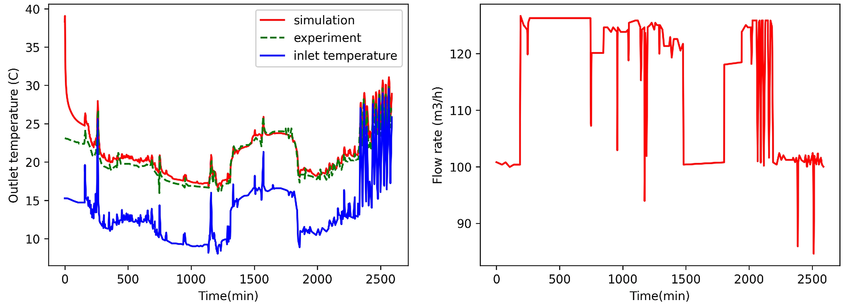
Figure 6. Comparison of simulated and measured outlet temperature of deep coaxial BHE array with center tube as inlet and annulus tube as outlet.
2.3 Economic model
2.3.1 Investment cost
(1) Unit Cost Model for Borehole Drilling
(1.1) Shallow Borehole Heat Exchanger Drilling Cost
The drilling cost of shallow borehole heat exchangers is significantly affected by various factors, making it difficult to obtain a fixed and unified value. The main influencing factors are as follows.
Geological conditions: If the geological structure of the construction area is dominated by hard rocks such as granite and basalt, professional rock drilling equipment, including down-the-hole drills, shall be adopted during drilling construction. Such conditions lead to heavy equipment wear and low construction efficiency, resulting in a substantial rise in drilling cost. The cost per meter may range from 200 to 500 RMB or even higher. By comparison, drilling operations in soft geological areas such as clay and sand strata can be completed with ordinary auger drills. Both equipment investment and construction difficulty are relatively low, and the drilling cost per meter is about 50 to 150 RMB.
Drilling depth: In general, the drilling cost presents an upward trend as the drilling depth increases. This is because the technical difficulty of drilling rises with greater depth, and complex underground conditions need to be addressed, including variations in formation pressure and groundwater leakage. Meanwhile, equipment wear will be aggravated, and more advanced equipment and technologies may be required to guarantee smooth drilling construction. For example, for shallow drilling within 100 meters, the cost per meter ranges from 100 to 200 RMB; when the drilling depth reaches 100-200 meters, it may increase to 150-300 RMB.
Pipe diameter and borehole diameter: The larger the pipe diameter and borehole diameter, the more pipe materials are required, and the higher the requirements for drilling equipment, which will increase the cost. To adapt to larger pipe diameters, the borehole diameter also needs to be increased, which raises the drilling workload and construction difficulty and further pushes up the cost.
Regional differences: Variations in economic development, labor cost and market competition among different regions will result in obvious differences in drilling costs. In economically developed areas, such as first-tier cities including Beijing, Shanghai, Guangzhou and Shenzhen, labor costs and equipment rental fees are relatively high. The drilling cost of shallow borehole heat exchangers in these regions may be 20%-50% higher than that in less developed areas. In regions with a weak industrial foundation and scarce resources, extra costs will be added as relevant equipment and materials need to be transported from other places.
(1.2) Medium-Deep Borehole Heat Exchanger Drilling Cost
The unit drilling cost of medium-deep boreholes (RMB/m) is related to drilling depth, formation hardness, and drilling equipment technology. The fitting calculation formula provided in the literature is used, as shown in Equation (11)[21]. This formula is derived from market survey data on borehole heat exchanger drilling costs in Shandong Province collected in Reference. The original data are unit costs (RMB/m) for boreholes at different depths, based on which the fitting formula is obtained.
Where κ denotes the drilling difficulty coefficient, with a value ranging from 1 to 2 (the default value of κ is set to 1.0); and H represents the drilling depth.
(2) Ground Horizontal Pipe Unit Cost Model
The surface section of borehole heat exchangers is generally provided with horizontal pipelines. There are two methods for calculating the cost of a single horizontal pipeline by using Equation (12)[27].
First, the cost is calculated via Equation (12). This cost is derived from data given in literature, and the pipe material adopts prefabricated polyurethane.
Where
Second, the horizontal pipe cost provided by engineering projects is directly adopted. This method is applicable to the analysis of both shallow and medium-deep borehole heat exchangers, and there is no need to invoke the fitting formula.
(3) Total Cost Model of Borehole Heat Exchangers
The total cost of borehole heat exchangers includes drilling cost, casing material cost and horizontal pipeline cost, which is calculated by Equation (13).
Where Nw denotes the number of borehole heat exchangers, and H is the drilling depth, m.
(4) Equipment Initial Investment Cost Model
The equipment initial investment mainly includes GSHP units, water pumps, cooling towers, air source heat pumps and boiler equipment, which is calculated by Equation (14).
Where Qhp is the designed capacity of the heat pump unit (kW), Chp is the unit power cost of the heat pump unit (RMB/kW), Qw is the power of the water pump (kW), Cwp is the unit power cost of the water pump (RMB/kW), Qeb is the designed capacity of the electric boiler unit (kW), Ceb is the unit power cost of the electric boiler unit (RMB/kW), Qgb is the designed capacity of the gas boiler unit (kW), Cgb is the unit power cost of the gas boiler unit (RMB/kW), ηeb and ηgb are the efficiencies of the electric boiler and gas boiler respectively, Qashp is the designed capacity of the air source heat pump (kW), Cashp is the unit power cost of the air source heat pump (RMB/kW), the coefficient 1.2 in the formula is a 120% redundancy design factor for the selected designed capacity, Qct is the designed capacity of the cooling tower (kW), and Cct is the unit capacity cost of the cooling tower (RMB/kW).
(5) Equipment Room Construction Cost Model
The equipment room construction cost Cro is related to the size and equipment of the machine room, which is calculated by Equation (15).
Where Qh is the user-side load, and Cro is the construction cost per unit load.
(6) Expansion of Grid Cost Model
Since all equipment is connected to the power grid, the power expansion cost Cp is calculated by Equation (16).
Where Php, Peb, Pgb, Pashp, Pct, Pwp are the operating powers of the GSHP, electric boiler, gas boiler, air source heat pump, cooling tower and water pump respectively, and cp is the unit power cost of power expansion, RMB/kW.
(7) Calculation Method of Other Costs
Other additional costs are estimated at 1% to 3% of the total cost.
2.3.2 Operation cost
The equipment operating cost is uniformly calculated by multiplying the equipment power consumption P (kW) by the electricity price Ce (RMB/kWh). The equipment power consumption includes that of heat pumps, water pumps and auxiliary cold and heat source equipment, which are calculated separately.
(1) Heat Pump Energy Consumption
In the GSHP system, heat pump energy consumption is the main component of the system. Its energy efficiency is closely related to the coefficient of performance (COP) of the unit. Equation (17)[28] is used to calculate the COP of the heat pump for cooling and heating operations. T represents the outlet water temperature of buried pipes, i.e. the water temperature entering the condenser under cooling condition and the evaporator under heating condition.
On the basis of COP calculation, the relational Equation (18) can be established between the user-side cold/heat loads and the ground-source side cold/heat loads. It is stipulated that the heating loads take positive values and the cooling loads take negative values; the subscript g represents the ground-source side, and the subscript user represents the user side.
To avoid the decrease in computational efficiency caused by excessive (if) conditional judgments in computer programs, Equation (19) is used for the unified calculation of heat pump power consumption, where mode = 0 represents cooling operation and mode = 1 represents heating operation.
(2) Water Pump Energy Consumption
Another source of power consumption during system operation is the water pump. Its power consumption is mainly calculated according to the pump head. The along-path hydraulic loss and local hydraulic loss are calculated by Equation (20) and Equation (21), respectively, and the power consumption (W) is subsequently calculated by Equation (22).
Where g is the gravitational acceleration, qm is the circulating mass flow rate (kg/s), and ηwp is the efficiency of the water pump.
(3) Energy Consumption of Auxiliary Cold and Heat Source Equipment
When the system provides cooling and heating for the user side, the GSHP cannot fully cover the load demand. Therefore, it is necessary to configure auxiliary heat sources (electric boiler, gas boiler, or air source heat pump) and cold source equipment (cooling tower cooperating with heat pump unit or air source heat pump).
(a) The energy consumption Pfs of auxiliary heat source equipment (electric boiler, gas boiler and air source heat pump) is calculated by Equation (23).
Where Qh,user represents the user-side heating load, RHS is the heating guarantee rate of the GSHP, and η is the efficiency of the corresponding auxiliary heat source equipment. The value of 0.9 is adopted for boilers, and the COP value is adopted for the air source heat pump.
(b) The energy consumption Pfs of auxiliary cold source equipment, including water-cooled heat pump and air source heat pump, is calculated by Equation (24).
Where Qc,user represents the user-side cooling load, RHS is the cooling guarantee rate of the GSHP, and η is the efficiency of the corresponding auxiliary cold source equipment. For air source heat pumps or water-cooled heat pump units, their COP values are adopted.
2.3.3 Index calculation
Economic performance evaluation indicators for geothermal-based heating and cooling systems over the full life cycle can be calculated by adopting total cost, average energy efficiency cost, investment PP, static rate of return and IRR. The indexes used in the study include: Dynamic Payback Period, Levelized Cost, Levelized Operating Cost, Initial Investment, Internal Rate of Return, and Profit Margin.
(1) Total Income (TIC)
TIC is calculated as shown in Equation (25).
Where ICi is the system investment in year i, OCi is the operating cost in year i, including annual electricity charges, fuel costs and equipment maintenance costs of each device. REi is the revenue in year i, including income from heating and cooling supply. For geothermal heating and cooling systems, a higher TIC over the full life cycle is preferred.
(2) NPV over Life Cycle
NPV is calculated as shown in Equation (26).
Where r is the discount rate, generally set at 8%. This discount rate is commonly adopted to convert future cash flows into present values, and supports customized settings in the program. RCny denotes the salvage value at the end of the full life cycle. For geothermal heating and cooling systems, a higher full life cycle NPV is preferred.
(3) Levelized Cost of Heating/Cooling (LCOHC)
LCOHC is an indicator measuring the average cost of unit heating and cooling capacity (e.g. kWh heat, kWh cold) of the system over the full life cycle. It is adopted for horizontal economic comparison among different heating and cooling technologies, including conventional air conditioning, ground source heat pumps, air-source heat pumps, etc. Its core logic is to convert the whole life cycle costs (initial investment, operating costs, etc.) into present value at the discount rate, and then allocate them to the total heating and cooling supply capacity, so as to reflect the long-term average economic cost per unit heating and cooling supply.
The calculation formula for LCOHC is given by Equation (27).
Where Qh,t and Qc,t are the hourly user-side heating load and cooling load, respectively.
Since the operating cost of the energy system has a significant impact on the overall levelized cost, the system operating cost is extracted separately to define a levelized operating cost.
(4) PP
PP is an economic evaluation indicator that measures the time required for an investment project to recover its initial investment. It reflects the capital recovery speed of the project and serves as a commonly used short-term benefit analysis tool in investment decision-making. Its core logic is to calculate the time point when the cumulative net cash flow changes from negative to zero, namely the number of years required to fully recover the initial investment.
According to whether the time value of capital is considered, the PP is divided into two types:
1. The static PP (without considering the time value of capital) is calculated directly based on the original amount without discounting future cash flows, and its formula is expressed as: static PP in a certain year = the year in which cumulative net cash flow turns positive - 1 + absolute value of cumulative net cash flow of the previous year/net cash flow of the current year, where net cash flow refers to current-year cash inflows including project revenue and sales income minus cash outflows including operating costs and maintenance costs, and cumulative net cash flow refers to the total sum of net cash flows from the initial stage of the project to year t.
2. The dynamic PP (considering the time value of capital) is obtained by converting future cash flows into present value at the discount rate (e.g. benchmark yield rate) and then calculating the time when the cumulative present value reaches zero, and its formula is: dynamic PP in a certain year = the year when cumulative NPV turns positive - 1 + absolute value of cumulative NPV of the previous year/NPV of the current year.
(5) IRR
IRR is a core dynamic indicator used to measure the investment profitability of a project. It represents the discount rate at which the NPV of the project equals zero throughout the entire calculation period. This indicator takes the time value of money into consideration, intuitively reflects the inherent profitability of the project, and is one of the key indicators commonly applied in investment decision-making.
The essence of the IRR is to solve for the discount rate (IRR) at which the project NPV equals zero. The formula is as follows.
Where NCFt represents the net cash flow in year t (cash inflow minus cash outflow); t represents the year (t = 0 refers to the initial investment period); n represents the project calculation period (including the construction period and operating period).
Calculation Method:
As the above formula is a higher-order equation, it cannot be solved directly by algebraic methods. In practice, IRR is generally estimated via the trial-and-error method (linear interpolation method), with the procedures as follows:
1. Estimate two discount rates r1 and r2:
Estimate two discount rates r1 and r2 such that the corresponding NPVs satisfy NPV1 > 0 (positive NPV at a lower discount rate) and NPV2 < 0 (negative NPV at a higher discount rate); in addition, the difference between r1 and r2 shall not be too large (generally no more than 5%) to ensure calculation accuracy.
2. Approximately calculate IRR using the linear interpolation method:
Assume that IRR lies between r1 and r2, and an approximate linear relationship exists between NPV and discount rate. The formula is as follows.
(6) Profit Rate
The formula is as follows.
2.4 Carbon emission model
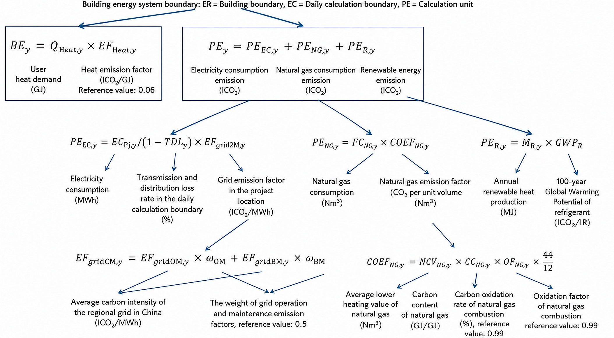
Geothermal systems (both medium-deep and shallow geothermal systems) are calculated in accordance with the calculation methodologies specified in Methodology for Voluntary Greenhouse Gas Emission Reduction Projects–Medium-deep Geothermal Energy Downhole Heat Exchange Heating Technology Application Project (CCER—01—003—V01), jointly issued on December 26, 2025 by the General Office of the Ministry of Ecology and Environment of China, the General Office of the Ministry of Housing and Urban-Rural Development, and the General Department of the National Energy Administration. All subsequent calculations comply with the stipulated calculation boundaries illustrated in Figure 7.
2.5 Optimization algorithm
Usually, the genetic algorithm is used for optimization of geothermal systems[29] or with aid of deep learning methods[30]. However, some optimization studies considering long-term operation of geothermal system can only optimize limited system parameters[31]. This study provides a better way of life cycle optimization of hybrid geothermal system.
BOA is a probabilistic model-based global optimization method, mainly used to solve optimization problems of high-dimensional, non-convex and computationally expensive black-box functions. Its core idea is to construct a probabilistic model (namely surrogate model) for the objective function, and combine it with an acquisition function to guide the selection of subsequent sampling points, so as to efficiently find the optimal solution of the objective function.
The procedure of Bayesian Optimization can be summarized as follows:
1. Initialization: Select a small number of initial sampling points within the domain of optimization variables, and calculate their objective function values.
2. Construct the surrogate model: Based on existing samples, a probabilistic model (usually Gaussian process (GP) is used to model the objective function, so as to obtain the posterior distribution of the objective function.
3. Select the next sampling point: Determine the most promising next sampling point from the domain by maximizing the acquisition function.
4. Update the sample set: Calculate the objective function value of the new sampling point and add it to the sample set.
5. Convergence judgment: If the convergence condition is satisfied (e.g., the maximum number of iterations is reached or the objective function value is sufficiently optimal), terminate the iteration; otherwise, return to Step 2.
Surrogate model (probabilistic model): It is adopted to approximate the behavior of the objective function f(x), among which GP is the most commonly used model. GP models the uncertainty of the objective function by assuming that the objective function follows a multivariate normal distribution, and is defined as:
where m(x) is the mean function, and k(x,x’) is the kernel function (used to characterize the correlation between sampling points). Given the dataset D = {(x1, y1), (x2, y2), …, (xn, yn)}, in which yi = f(xi) + ϵ and ϵ represents noise, the posterior distribution of the objective function value f(x*) at a new query point x* is a normal distribution:
where μ(x*) is the posterior mean (representing the predicted value of f(x*)), and σ2(x*) is the posterior variance (representing the prediction uncertainty).
Acquisition Function: It is used to balance exploration (exploring high-uncertainty regions) and exploitation (utilizing known high-performance regions). Commonly used acquisition functions include:
Expected improvement (EI):
where xbest is the current known optimal sampling point, and f(xbest) is its objective function value. This function measures the EI that the objective function value at a new point x surpasses the current optimal value.
Probability of improvement:
where ξ is a small positive constant, which controls the degree of exploration. This function represents the probability that the objective function value at a new point x is better than the current optimal value.
Upper confidence bound:
where κ is the trade-off coefficient, which adjusts the emphasis placed on the mean (exploitation) and variance (exploration).
The main advantages of Bayesian Optimization are as follows: it does not require derivative information of the objective function and is suitable for black-box function optimization; it quantifies uncertainty through the probabilistic model, so as to efficiently utilize existing information and reduce unnecessary sampling; and it exhibits high optimization efficiency for computationally expensive functions (e.g., engineering simulation and hyperparameter tuning). By dynamically updating the surrogate model and reasonably selecting acquisition functions, Bayesian Optimization can rapidly approach the global optimal solution with limited computational resources, and thus serves as an important tool for complex optimization problems.
2.6 Cases and boundaries
Xi’an is selected as the case study area for calculation. District heating loads are undertaken by middle-deep geothermal borehole heat exchangers, ASHP and gas-fired boilers, and the heating load allocation ratios of the three devices are to be optimized. District cooling is solely supplied by ASHP because this is a cold region where space heating dominates and usually caused huge carbon emissions. In accordance with the latest national standard GB/T 18430.1-2024, the cooling COP of comfort units shall not be less than 2.8. Therefore, a cooling COP of 3.0 is adopted for calculation in this case. According to data provided by equipment manufacturers, the unit price of air-source units ranges from 1.0 to 1.5 yuan/W, and the unit price of 1.5 yuan/W is adopted in this study.
When gas-fired boilers are involved in district heating supply, the natural gas pipeline network shall be expanded or retrofitted during project construction in accordance with the daily peak natural gas consumption of the region. Accordingly, a certain expansion fee needs to be paid to the natural gas company, which is generally charged at 400-600 yuan/m3. In addition, energy stations are characterized by large electrical load demand, so power grid expansion costs shall be taken into account during construction. There is no unified national charging standard. By referring to the Budget Quota for Electric Power Engineering Construction (2021 Edition), industrial power connection project charging standards issued by provincial and municipal power companies, and practical market engineering, procurement, and construction general contracting cases of energy stations, a typical example is the tender announcement for the 10 kV substation project of Changzhou Xinlong Phase II Energy Main Station. Its core parameters include two 2,000 kVA dry-type transformers, 10 kV dual power supply and cable incoming line, with a total project cost of about 2.4 million yuan (equivalent to 1.2 yuan/W). Power grid expansion fees are generally charged by voltage level: Low voltage (380 V): 0.5-1.8 yuan/W; Medium voltage (10 kV): 0.9-3.0 yuan/W; High voltage (35 kV): 1.4-4.6 yuan/W; and Ultra-high voltage (above 110 kV): 1.3-4.2 yuan/W.
In terms of charging standards, the district heating tariff for residential buildings is 23.2 yuan per square meter per heating season, and the district heating tariff for public buildings is 30 yuan per square meter per heating season. Central cooling service is not provided for residential buildings, while the district cooling tariff for public buildings is 30 yuan per square meter per cooling season, and the cooling period is calculated as 4 months. The main calculation parameters adopted for the heating optimization design are summarized in Table 1.
Table 1. Calculation parameters for heating optimization design of medium-deep geothermal systems in Xi’an.
| Parameters | Value | Parameters | Value |
| Equipment Room Construction Cost | 1.0 yuan/W | Personnel Cost | 3,700 yuan/month |
| Number of Personnel | 3 persons | Annual Equipment Maintenance Cost | 1% of equipment investment cost |
| Heating Area | 200,000 m2 | System Service Life | 30 years |
| Default Material of Central Pipe | DN110 Heat-Resistant Polyethylene Pipe for Hot and Cold Water | Default Material of Outer Casing Pipe | Oil Casing |
| Comprehensive Installation Cost of Casing Pipe | 0 yuan/m | Drilling Cost | Below 2,500 m: 800 yuan/m Above 2,500 m: 940 yuan/m |
| Comprehensive Cost of Surface Horizontal Pipeline | 10 yuan/m | Natural Gas Price | 2.89 yuan/m3 |
| Water Pump Efficiency | 0.9 | Unit Price of Water Pump | 0.045 yuan/W |
| Heat Pump Efficiency | 4.5 | Unit Price of Heat Pump | 0.58 yuan/W |
| Gas-Fired Boiler Efficiency | 0.9 | Unit Price of Gas-Fired Boiler | 0.25 yuan/W |
| Air-Source Heat Pump Efficiency | 2.5 | Unit Price of Air-Source Heat Pump | 1.5 yuan/W |
| Gas Distribution Network Expansion Cost | 800 yuan/m3 | Power Grid Expansion Cost | 3.0 yuan/W |
| Government Subsidy | Subsidy based on heating area: 120.8 yuan/m2 | District Heating Tariff | Residential buildings: 23.2 yuan/m2/heating season Public buildings: 25 yuan/m2/heating season |
| Subsidy based on the proportion of initial investment (not applicable to Xi’an) | District Cooling Tariff | No central cooling service is provided for residential buildings; the cooling tariff for public buildings is 25 yuan/m2/cooling season | |
| Electricity Price | 0.6 yuan/kWh |
Typical public and residential building models are developed using the TRNSYS software. The basic parameters of the residential building are presented in Table 2, with a floor area of 5,961 m2 per single unit. The occupancy and equipment operation schedules of the residential building on weekdays and weekends are listed in Table 3 and Table 4, respectively. Based on these parameter configurations, the hourly heating and cooling loads are simulated by applying the established models under the typical meteorological year conditions of Xi’an. The annual heating season commences on November 15 and concludes on March 15 of the subsequent year, spanning a duration of 121 days. As shown Figure 8, the per-unit-area load indices are derived first, and then multiplied by the total floor area of 200,000 m2 to obtain the full-scale system loads.
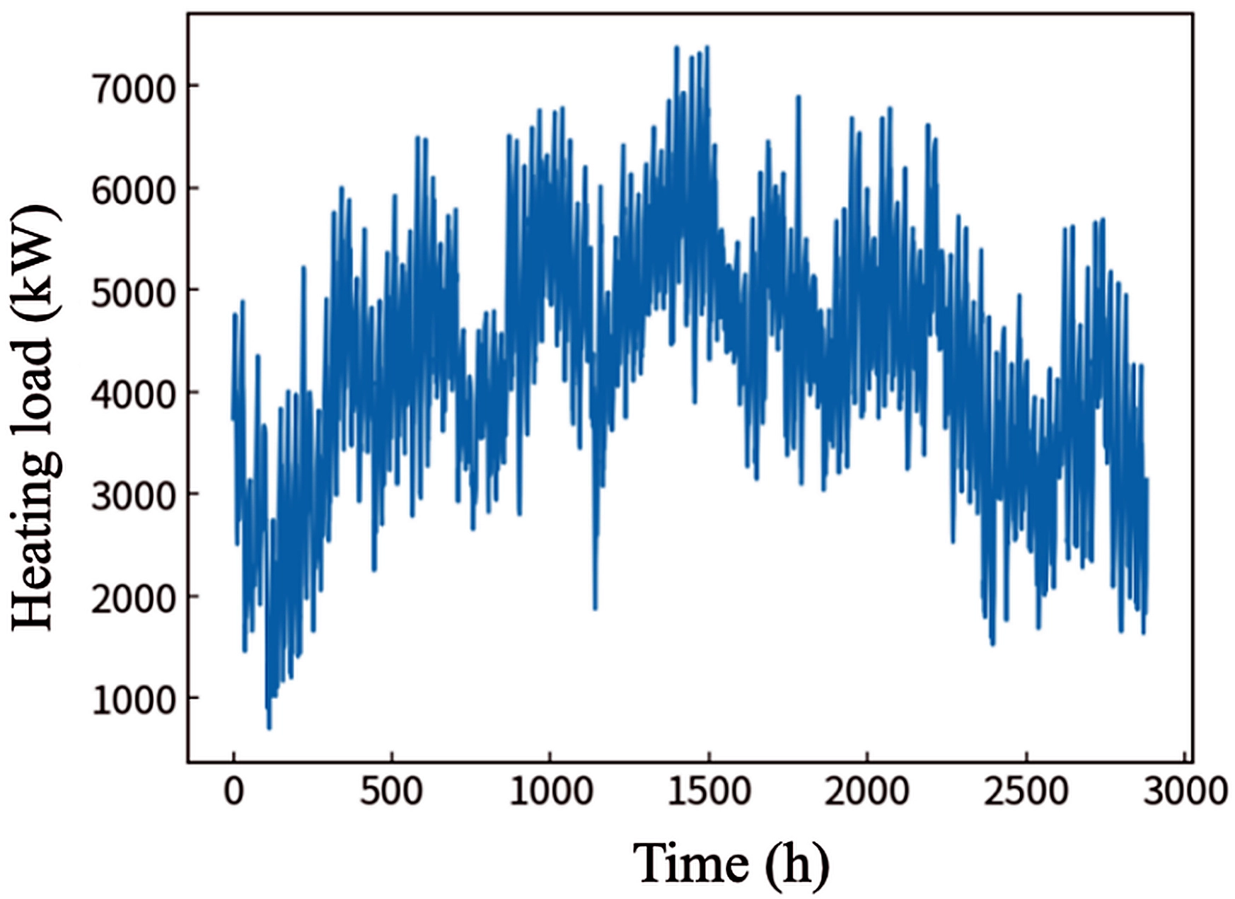
Table 2. Basic parameters of residential buildings.
| Parameters | Value | Parameters | Value |
| Height | 36.2 m | Window-to-Wall Ratio | 0.3 |
| Width | 19.49 m | Lighting Power Density | 6 W/m2 |
| Length | 25.49 m | Equipment Power Density | 4.3 W/m2 |
| External Wall U-value | 0.3 W/K*m2 | Occupancy Density | 0.03 person/m2 |
| Roof U-value | 0.2 W/K*m2 | Cooling/Heating Setpoint Temperature | 26/18 °C |
| External Window U-value | 2.0 W/K*m2 |
Table 3. Occupancy and equipment operation schedules for residential buildings on weekdays.
| Start Time | End Time | Occupancy | Fresh Air | Lighting | Equipment |
| 0 | 7 | 0.95 | 0 | 0.05 | 0.2 |
| 7 | 8 | 0.9 | 0 | 1.00 | 1.00 |
| 8 | 9 | 0.4 | 0 | 0.5 | 0.5 |
| 9 | 12 | 0 | 0 | 0.05 | 0.2 |
| 12 | 14 | 0.5 | 0 | 0.7 | 0.60 |
| 14 | 18 | 0 | 0 | 0.05 | 0.2 |
| 18 | 20 | 0.8 | 0 | 1.00 | 1.00 |
| 20 | 23 | 0.95 | 0 | 1.00 | 1.00 |
| 23 | 0 | 0.95 | 0 | 0.05 | 0.2 |
Table 4. Occupancy and equipmentoperation schedules for residential buildings on weekends.
| Start Time | End Time | Occupancy | Fresh Air | Lighting | Equipment |
| 0 | 7 | 0.95 | 0 | 0.05 | 0.2 |
| 7 | 8 | 0.9 | 0 | 0.5 | 0.5 |
| 8 | 9 | 0.8 | 0 | 1.00 | 1.00 |
| 9 | 12 | 0.5 | 0 | 0.7 | 0.8 |
| 12 | 14 | 0.95 | 0 | 1.00 | 1.00 |
| 14 | 18 | 0.5 | 0 | 0.7 | 0.8 |
| 18 | 20 | 0.8 | 0 | 1.00 | 1.00 |
| 20 | 23 | 0.95 | 0 | 1.00 | 1.00 |
| 23 | 0 | 0.95 | 0 | 0.05 | 0.2 |
In the subsequent calculations, simple processing is required for the hourly building load data of the entire year, as the summer cooling operating conditions also need to be analyzed simultaneously: (1) All winter heating load data shall be positive at every hour to ensure no cooling load occurs in winter; (2) All summer cooling load data shall be negative at every hour to ensure no heating load occurs in summer; (3) All loads during the transition seasons are set to 0, to correspond to the zero operating flow rate of pumps in these periods. The modified annual hourly loads of the public building in Xi’an are shown in Figure 8. Based on the characteristics of the load data, the year is divided into 120 days of winter, 51 days of spring, 120 days of summer, and 74 days of autumn; (4) This study requires a comprehensive economic analysis of both winter heating and summer cooling. Referring to load data of typical public or residential buildings in cold regions provided in relevant literature, the original loads need to be adjusted. In the preliminary design, the winter-to-summer load ratio is set to 1:1; at the data level, the winter heating load is directly replicated as the summer cooling load; (5) Statistics show (Figure 8) that the peak heating load index of the residential building in Xi’an is 36.8 W/m2, the peak load of the 200,000 m2 building is 7,378 kW, and the total heat supply per heating season is 224 GJ/m2.
3. Results and Discussions
3.1 Impact of non-design factors
3.1.1 Long-term thermal attenuation of medium-deep geothermal systems
Medium-deep geothermal borehole heat exchanger systems mainly operate during the heating season and recover thermally during the non-heating season. However, full recovery to the initial ground temperature is difficult to achieve, resulting in a gradual decline in ground temperature and outlet water temperature over long-term operation. Directly simulating 30 years of hourly heat transfer for each optimization iteration is computationally inefficient. Therefore, this study adopts a simplified approach in which the first-year heat transfer calculation is used, while the long-term attenuation effect is represented by increasing the lower limit of the inlet water temperature in the first year. It is found that under different borehole configurations, this higher bound value for the first-year temperature only varies within 2 degrees, causing a minor effect on the final evaluation indexes.
The 30-year simulation based on the hourly heating load of residential buildings in Xi’an shows that, for 12 medium-deep boreholes with a depth of 3,000 m and a single-well flow rate of 30 m3/h, the maximum difference in inlet water temperature between the first and the 30th heating seasons reaches 9.3 °C (Figure 9). Accordingly, if the inlet water temperature in the 30th year is required to remain above 4 °C, the minimum inlet water temperature in the first year should be no lower than 13.3 °C. In the subsequent optimization, a representative first-year inlet temperature limit is therefore adopted to account for long-term thermal attenuation.
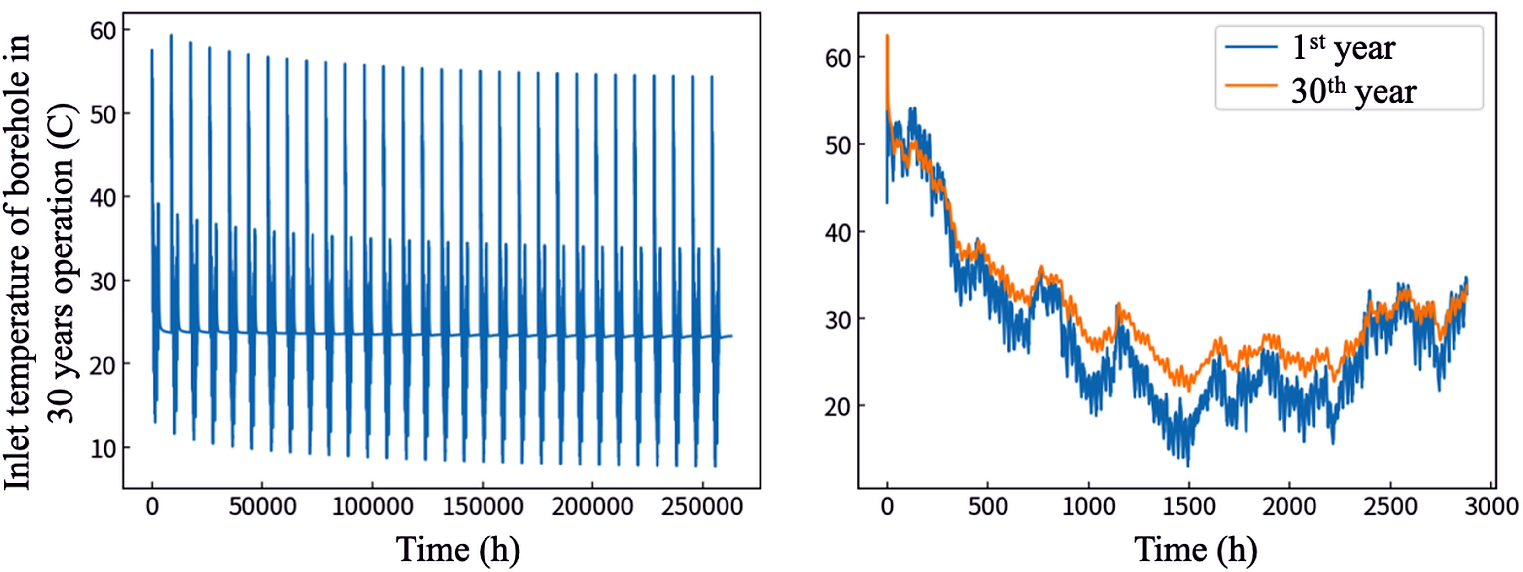
Figure 9. Long-term water temperature attenuation of middle-deep geothermal buried pipes.
Table 5 compares the optimization results under different lower-limit settings of inlet water temperature. The results show that neglecting thermal attenuation may lead to overly optimistic economic evaluations. When the inlet water temperature limit increases from 4 °C to 14 °C, the optimal PP increases by nearly two years. This demonstrates that long-term thermal attenuation should be incorporated into life-cycle economic analysis of medium-deep geothermal systems.
Table 5. Comparison of optimization results under different lower limit settings of inlet water temperature.
| First-Year Inlet Water Temperature Lower Limit | ||||||
| Optimal Parameter Configuration | 4 °C | 6 °C | 8 °C | 10 °C | 12 °C | 14 °C |
| Drilling Depth (m) | 3,350 | 3,200 | 3,300 | 3,300 | 3,450 | 3,500 |
| Number of Boreholes | 7 | 8 | 8 | 8 | 8 | 8 |
| Single Borehole Flow Rate (m3/h) | 41 | 37 | 36 | 41 | 45 | 39 |
| Optimal Payback Period (Year) | 8.14 | 8.81 | 9.03 | 9.31 | 9.67 | 9.75 |
3.1.2 User-side load uncertainty
User-side load uncertainty is another important non-design factor affecting system performance. In practical projects, the actual heating load may deviate from the design value due to variations in occupancy, building operation, and indoor thermal demand. To evaluate this effect, the user-side load is varied from 0.8 to 1.2 times the baseline load.
As shown in Table 6, load fluctuation has a significant impact on the optimal economic performance. Under the baseline load, the optimal PP is 9.75 years. When the actual load is 20% lower than the baseline, the PP decreases to 6.16 years; when the load is 20% higher, it increases to 14.64 years. Even a 10% load deviation can cause a difference of approximately 2-3 years in the PP.
Table 6. Considering long-term thermal attenuation of medium-deep geothermal systems (Tin_min = 14 °C).
| User-Side Load Fluctuation Ratio | |||||
| Optimal Parameter Configuration | 0.8 | 0.9 | 1.0 | 1.1 | 1.2 |
| Drilling Depth (m) | 3,300 | 3,450 | 3,500 | 3,450 | 3,450 |
| Number of Boreholes | 7 | 7 | 8 | 9 | 10 |
| Single Borehole Flow Rate (m3/h) | 42 | 48 | 39 | 40 | 37 |
| Optimal Payback Period (Year) | 6.16 | 7.78 | 9.75 | 12.22 | 14.64 |
Table 7 further evaluates the economic performance of the design parameters obtained under the baseline load ratio of 1.0 when applied to different actual load conditions. The results indicate that lower-than-design loads can maintain heating reliability and improve economic performance. In contrast, higher-than-design loads reduce the RHS value and worsen the overall economic indicators. Therefore, user-side load uncertainty should be carefully considered in the design and optimization of medium-deep geothermal systems.
Table 7. Economic performance of design parameters obtained under the load ratio of 1.0 when applied to actual load conditions.
| User-Side Load Fluctuation Ratio | |||||
| Economic Index | 0.8 | 0.9 | 1.0 | 1.1 | 1.2 |
| Payback Period (Year) | 7.86 | 8.76 | 9.75 | 10.84 | 11.96 |
| Levelized Cost (CNY/GJ) | 181.63 | 169.92 | 160.78 | 153.39 | 146.89 |
| Levelized Operating Cost (CNY/GJ) | 33.18 | 32.63 | 32.41 | 32.33 | 31.92 |
| Initial Investment (104 CNY) | 5,093 | 5,294 | 5,495 | 5,696 | 5,897 |
| Internal Rate of Return (%) | 14.27 | 12.46 | 10.85 | 9.42 | 8.20 |
| Profit Rate (%) | 147.93 | 131.75 | 116.31 | 101.75 | 88.96 |
| RHS | 1 | 1 | 1 | 0.8 | 0.69 |
RHS: ratio of heating supply.
3.2 Impact of design factors
3.2.1 Parameter analysis
Prior to the optimization design phase, key design parameters that significantly influence the economic indicators of medium-deep geothermal systems are analyzed individually to clarify their impact patterns. This analysis also establishes the upper and lower boundary values required for subsequent index normalization calculations. For the following analysis, the geothermal geological parameters, labor costs, maintenance fees, and other baseline parameters adopted in Section 2.6 are retained. The dimensions, thermophysical properties, and surface roughness of the central pipe and outer casing pipe are all based on pipe material datasheets for products manufactured by Canghai Mingzhu, which were collected through market surveys and literature research.
In the parameter analysis, residential buildings in Xi’an are selected as the default case. The baseline configuration is set as follows: a drilling depth of 2,000 m, 8 wells, a single well flow rate of 24 m3/h, DN110 heat-resistant polyethylene pipes for hot and cold water for all central pipe sections, and oil casing pipes for the outer casing. The installed capacity ratio is initially set to 50% for ground-source heat pump units and 50% for air-source heat pump units. The minimum inlet water temperature in the first year is set to 14 °C to account for the system’s 30-year operational thermal attenuation. Six economic indicators are adopted in the analysis: PP, levelized cost, levelized operating cost, IRR, total profit rate, and initial investment cost. In addition, the RHS curve of the system is plotted.
Note: In the subsequent optimization analysis, the RHS of the geothermal system is set to 1 as the basic constraint. If certain parameter combinations fail to realize cost recovery within the 30-year operation cycle, the program will automatically assign a PP of 100 years and a levelized cost of 1,000 CNY/GJ by substituting relatively large values. This approach creates an obvious penalty term for the minimization calculation, facilitating effective optimization in the follow-up calculation.
In this section, in addition to analyzing the influence trends of various design parameters on economic indicators, the monotonic variation characteristics of different economic indicators are summarized. Meanwhile, according to the variation rate of each indicator curve with independent design parameters, the sensitivity of each design parameter to the changes of economic indicators is defined.
3.2.2 Number of boreholes
A relatively wide parameter range is first adopted, with the number of geothermal wells set from 7 to 10. On this basis, six economic indicators and the system heating supply reliability are calculated, and the corresponding results are shown in Figure 10 and Figure 11. It can be observed that a configuration of 7 wells fails to fully cover the heating load demand of the geothermal system. Furthermore, an increase in the number of wells significantly prolongs the PP and raises the levelized cost, and the levelized operating cost also shows a slight upward trend with the growth of well quantity. Although the heating supply reliability is maintained at 1 for 8 to 10 wells, the power consumption of water pumps increases along with the rising number of wells, leading to a sharp decline in the overall profit rate.
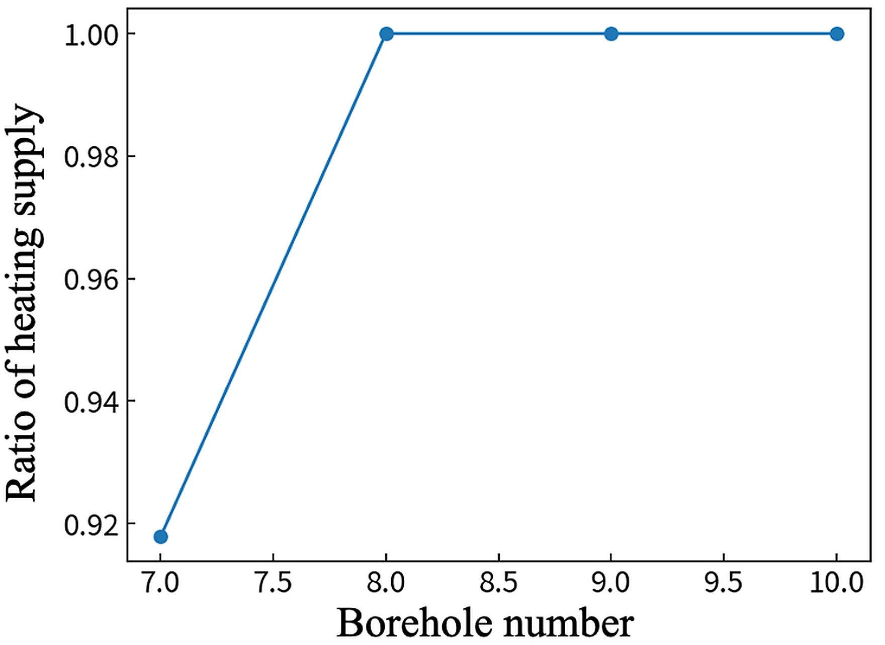
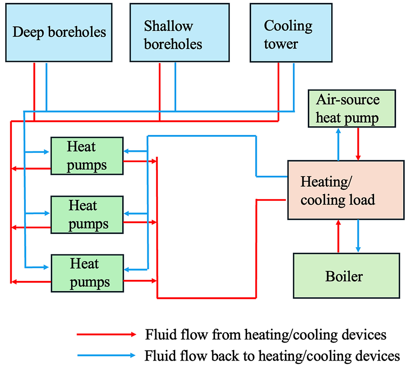
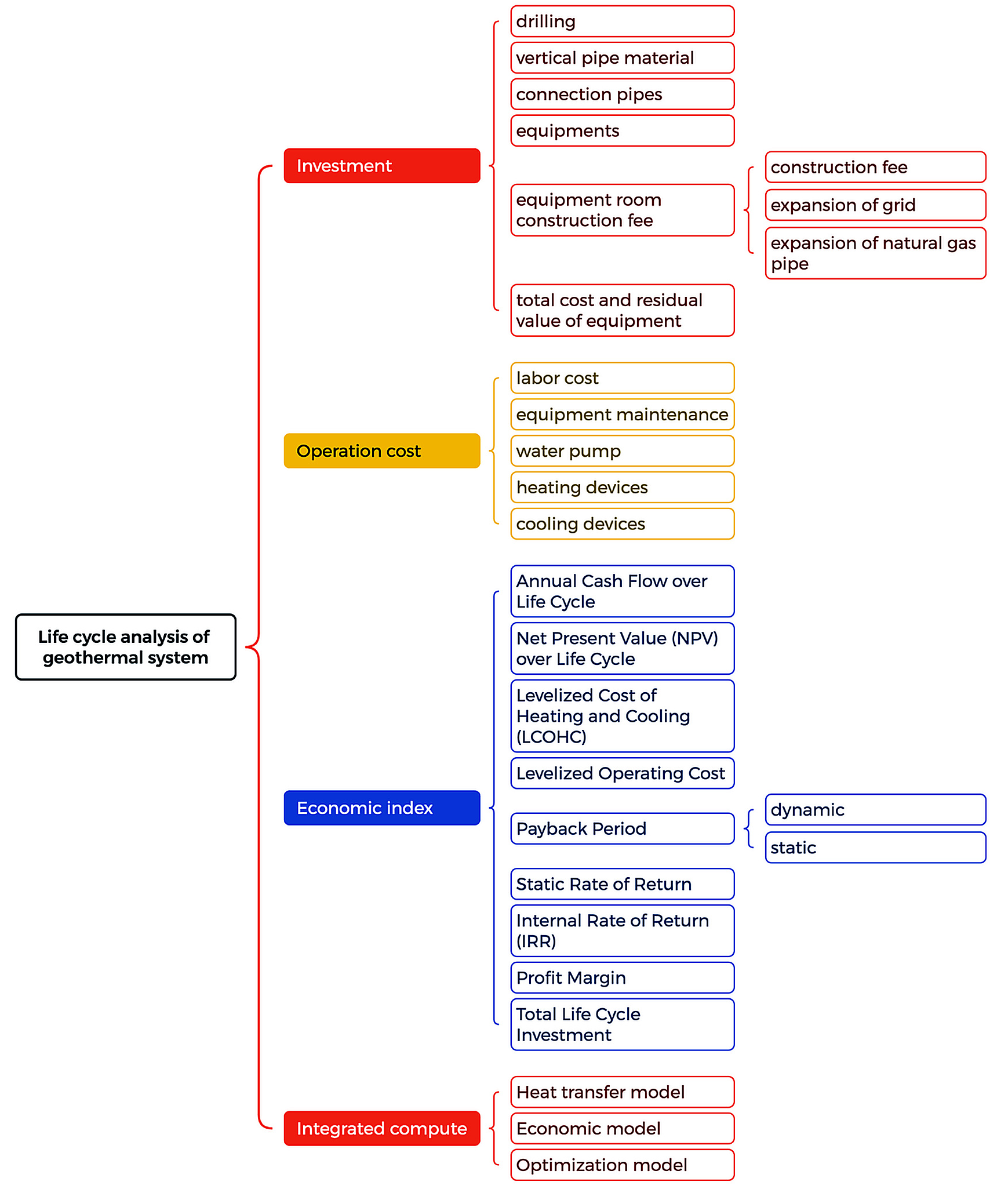
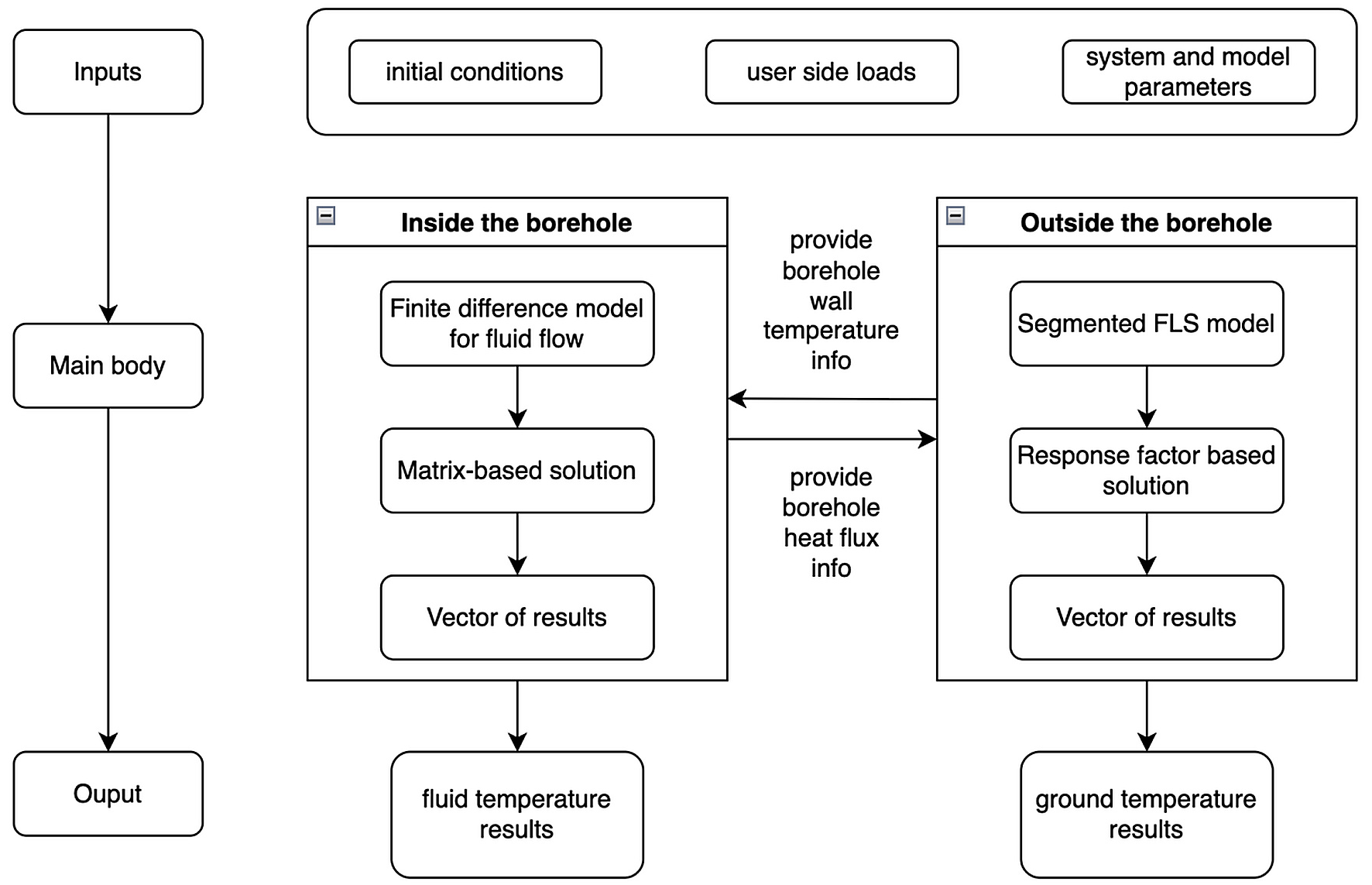
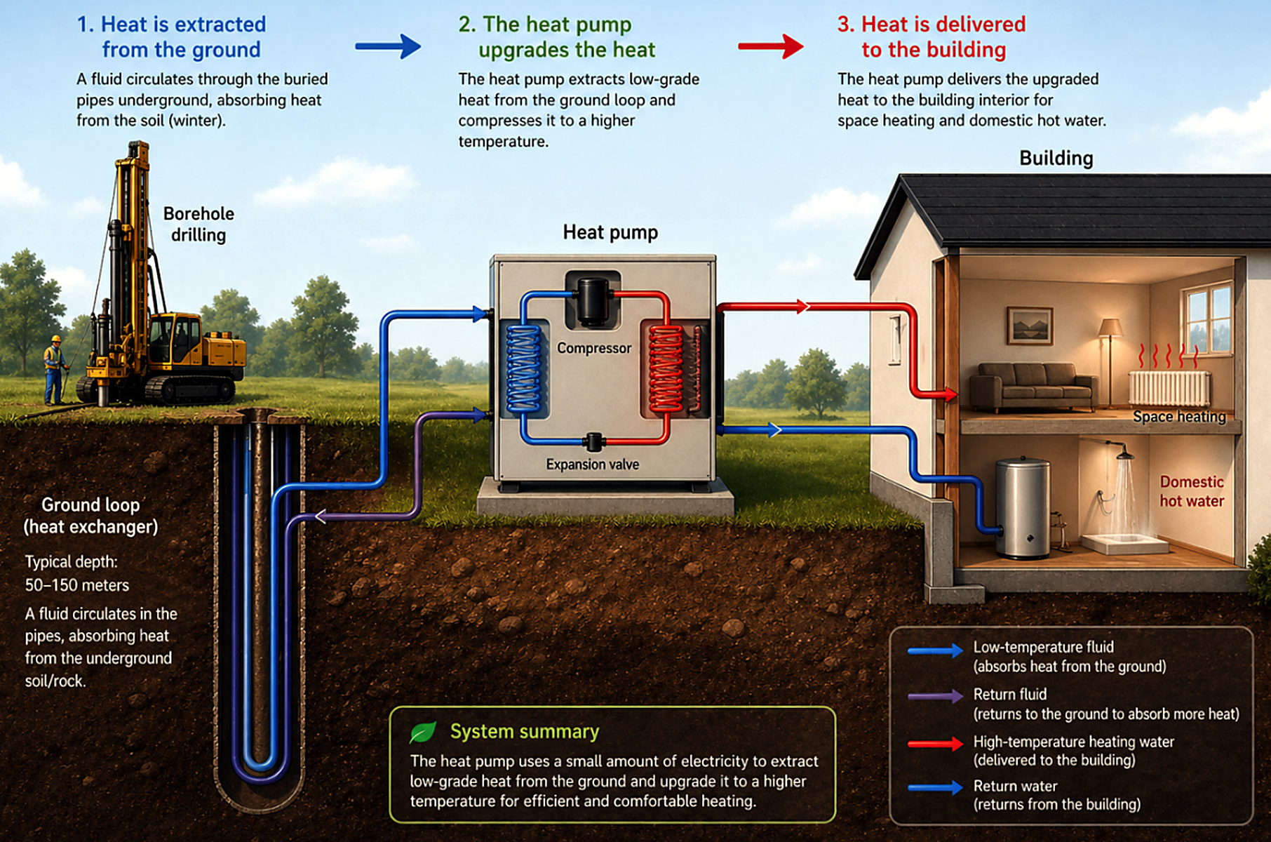
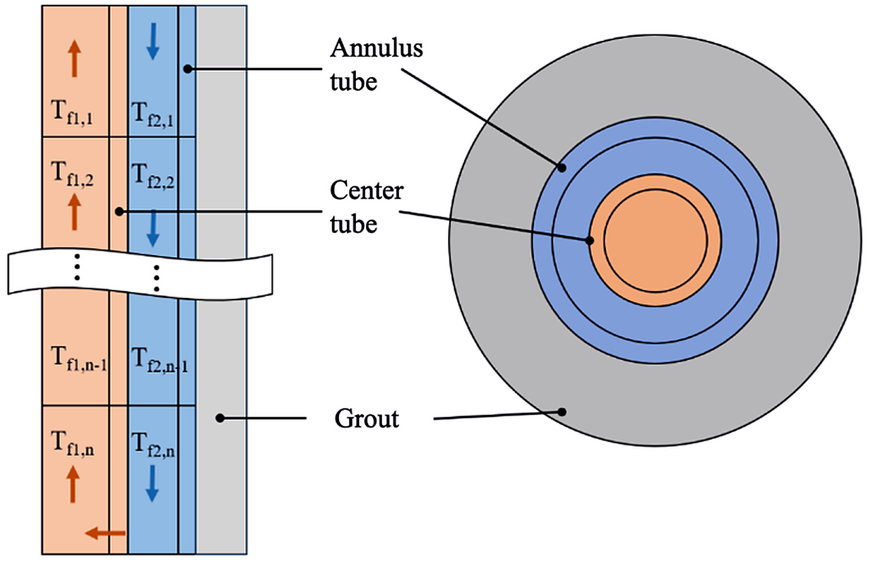
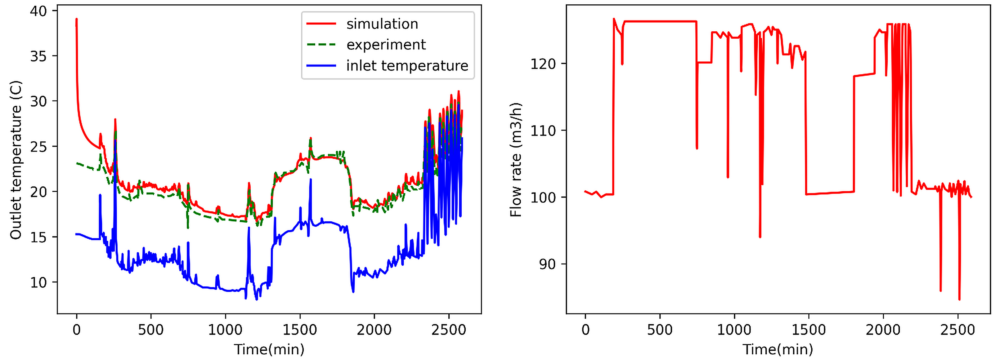
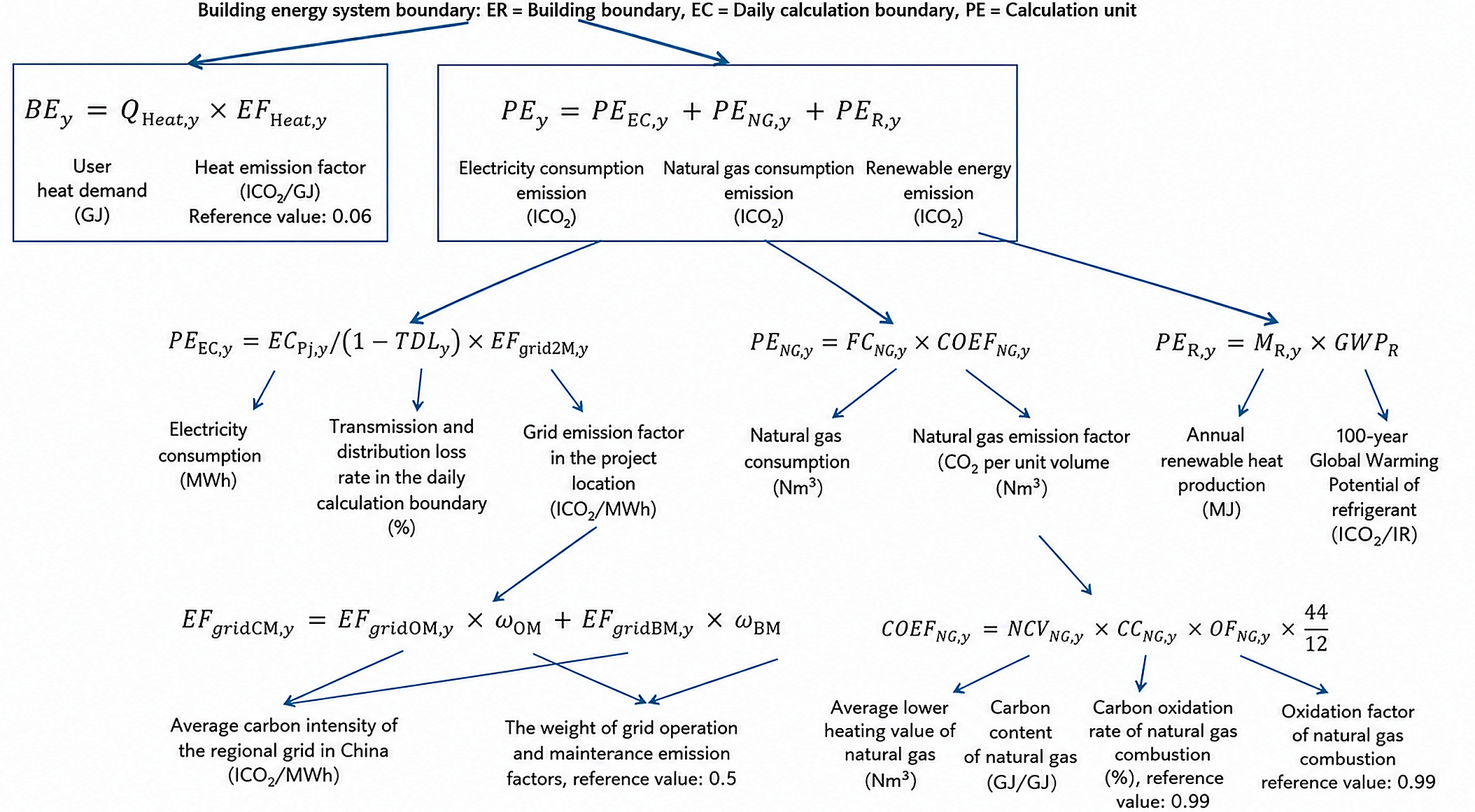
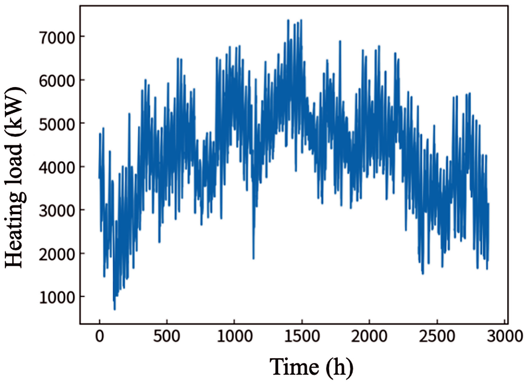
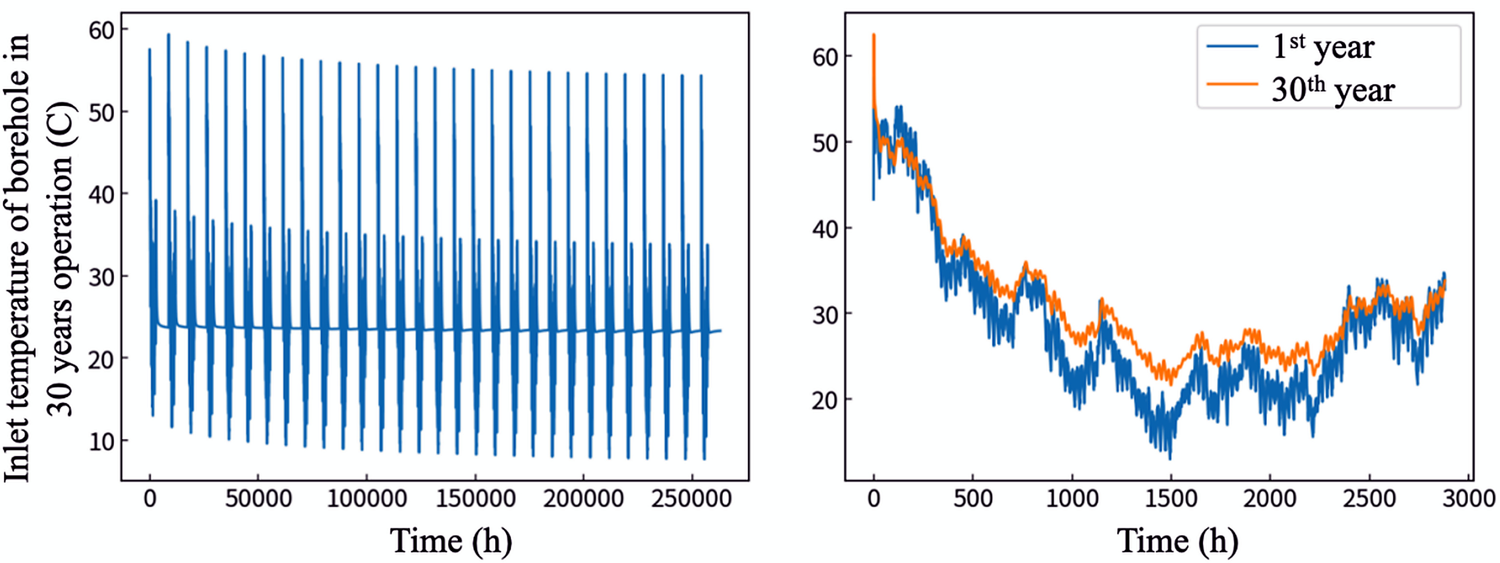
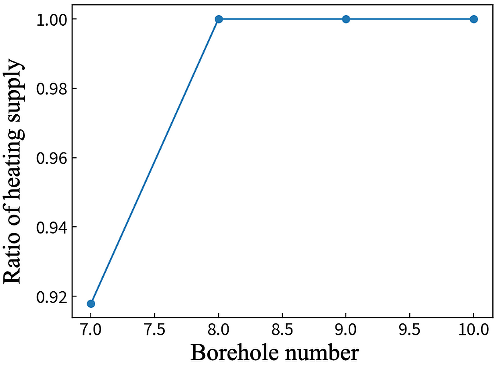
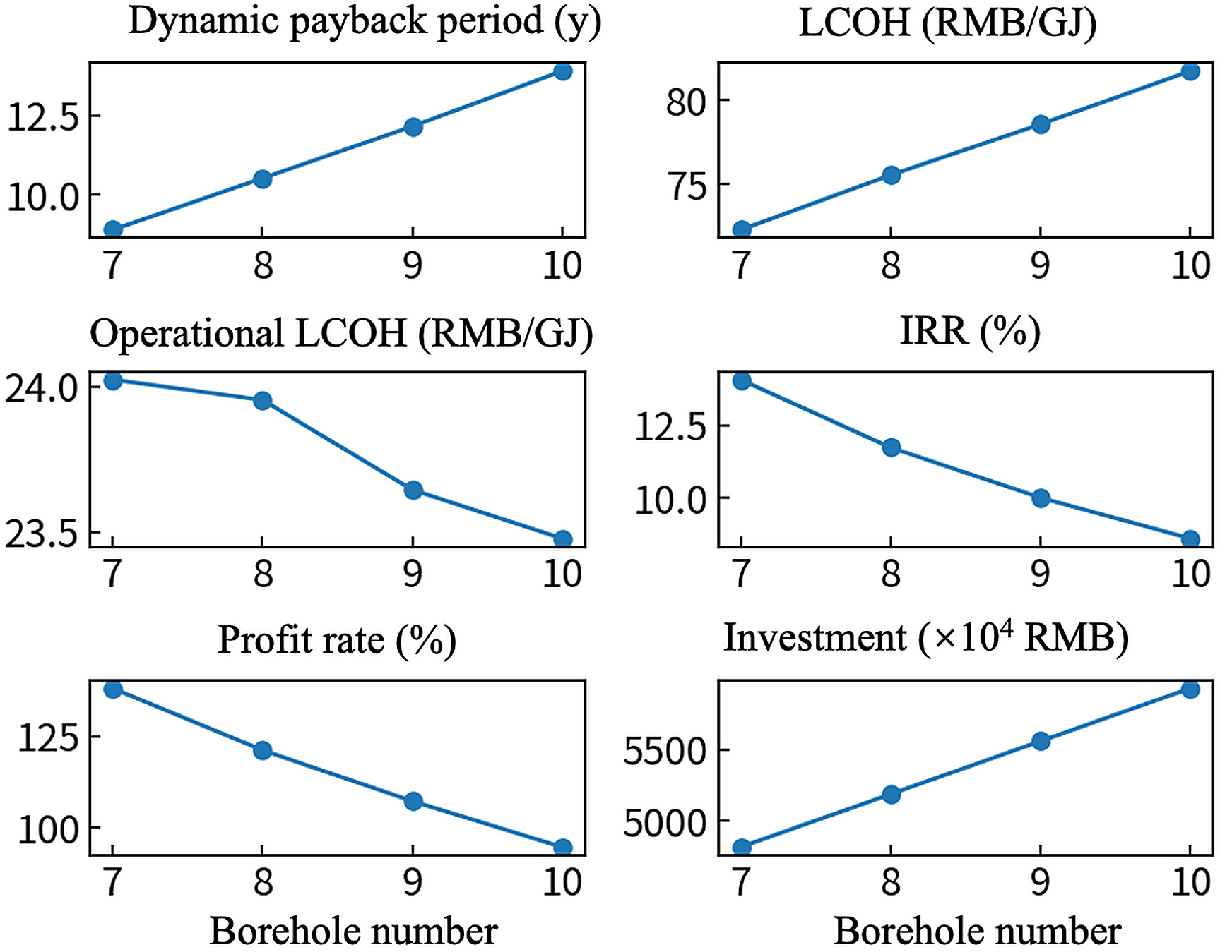
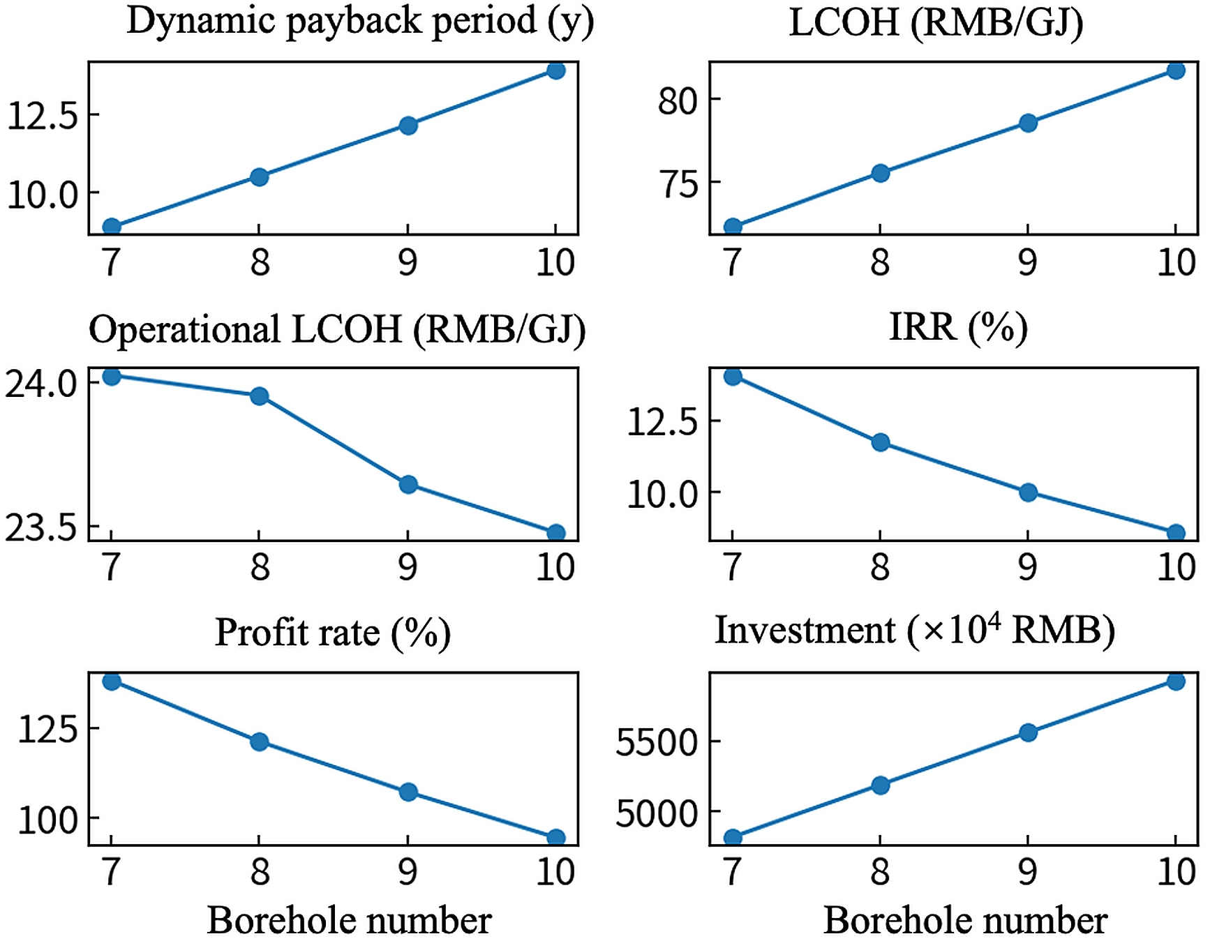
Figure 11. Influence of different borehole quantities on each index. LCOH: levelized cost of heating; IRR: internal rate of return.
3.2.3 Drilling depth
A reasonable range of drilling depth from 2,900 m to 3,500 m is selected firstly. Six economic indicators and the system RHS are calculated within this range, and the results are presented in Figure 12 and Figure 13. The RHS remains at 1 throughout the selected depth interval. As the drilling depth increases, the PP, levelized cost and initial investment rise continuously, while the profit rate, operating cost and IRR decline steadily. Since the RHS is fully satisfied under the current parameter settings, a deeper drilling depth delivers a higher outlet water temperature and improves the COP of the heat pump. With the total heating supply unchanged, the power consumption of the heat pump is thereby reduced.
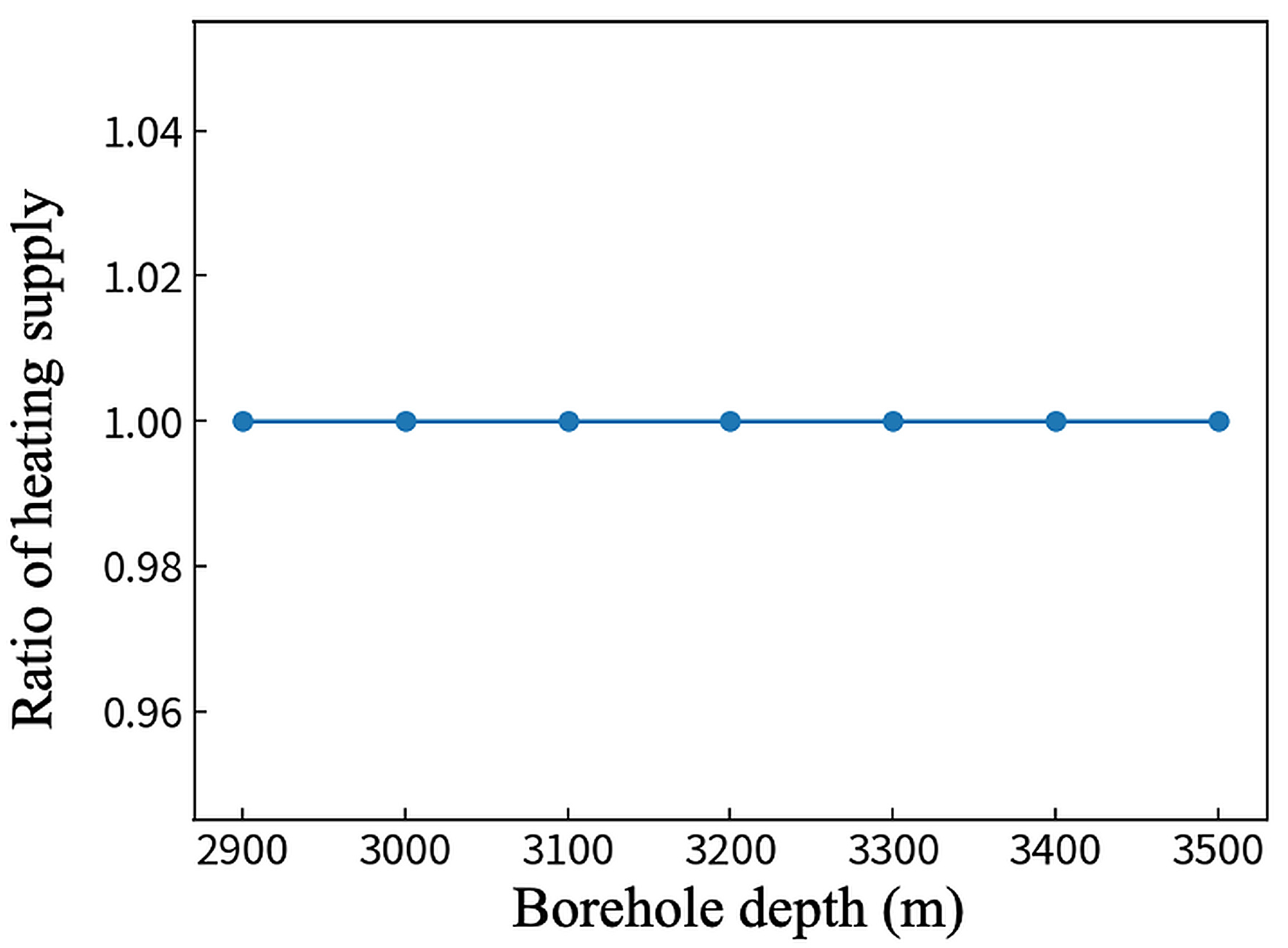
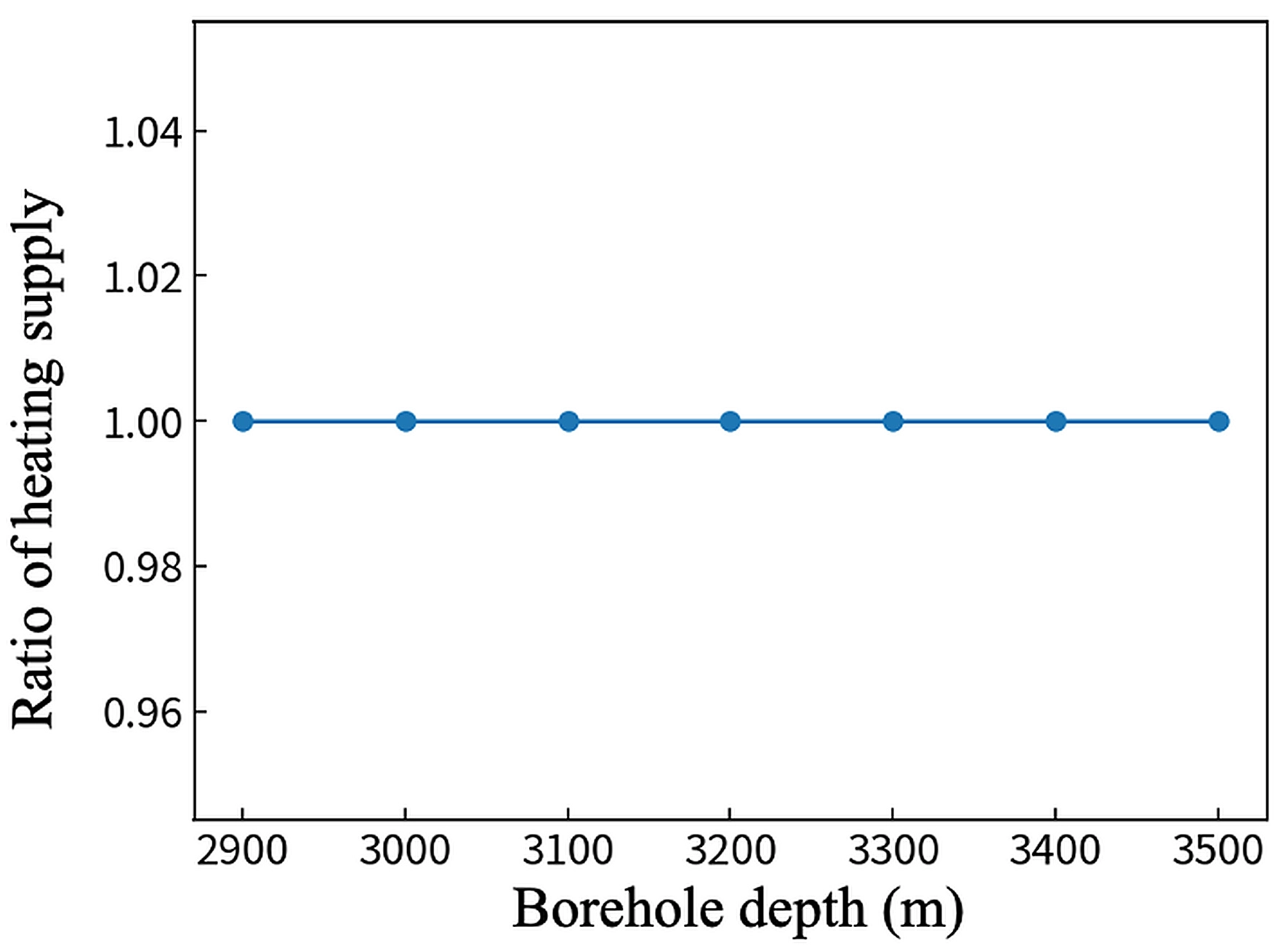
Figure 12. The RHS under different drilling depth settings. RHS: ratio of heating supply.
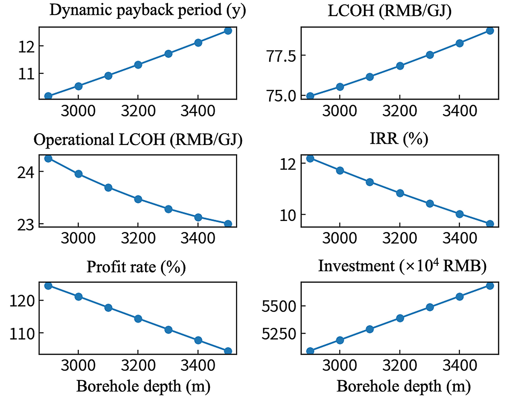
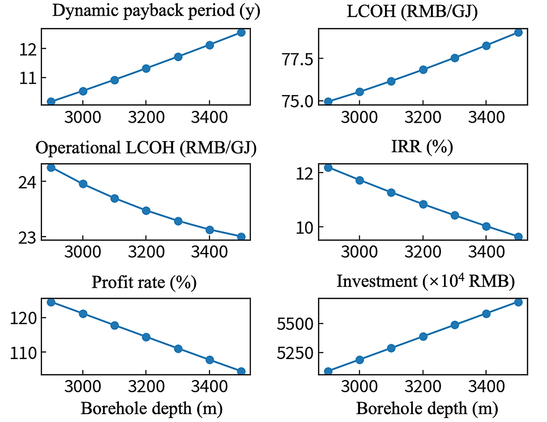
Figure 13. Influence of different drilling depth on each index. LCOH: levelized cost of heating; IRR: internal rate of return.
3.2.4 Single borehole flow
A reasonable range of single borehole flow rate is selected, including 20, 22, 24, 26, 28 and 30 m3/h. Six economic indicators and the system RHS are calculated accordingly, and the results are shown in Figure 14 and Figure 15. With the increase of single borehole flow rate, the RHS of the geothermal system rises continuously and eventually remains at 1, while the flow rate of 20 m3/h cannot guarantee 100% heating supply. Meanwhile, the PP, levelized cost and operating cost increase gradually, the profit rate decreases continuously, and the initial investment remains unchanged. Flow rate mainly affects the power consumption of water pumps and exerts little influence on heat pump units when the RHS is maintained at 1. Consequently, the normalized curves of system levelized cost and operating cost are nearly coincident.
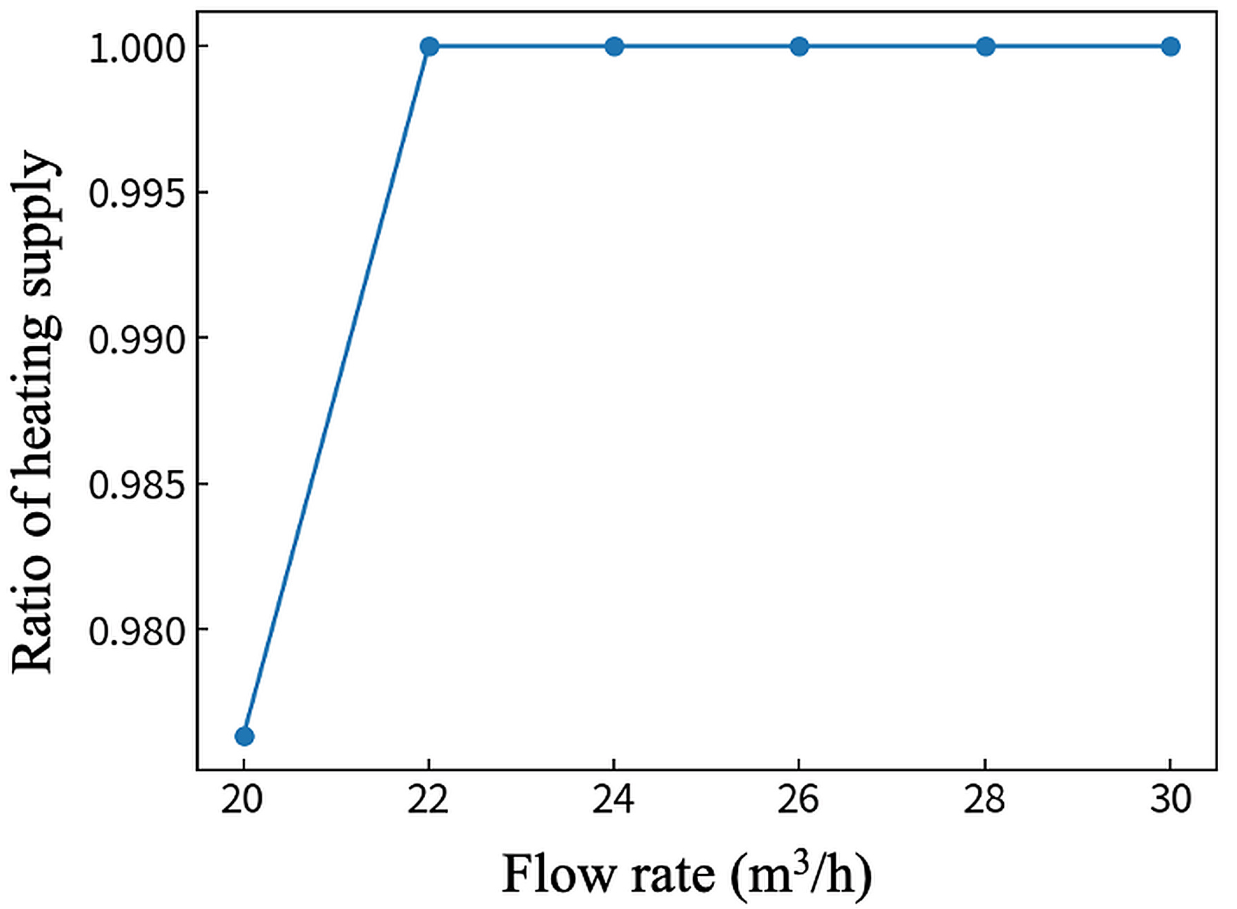
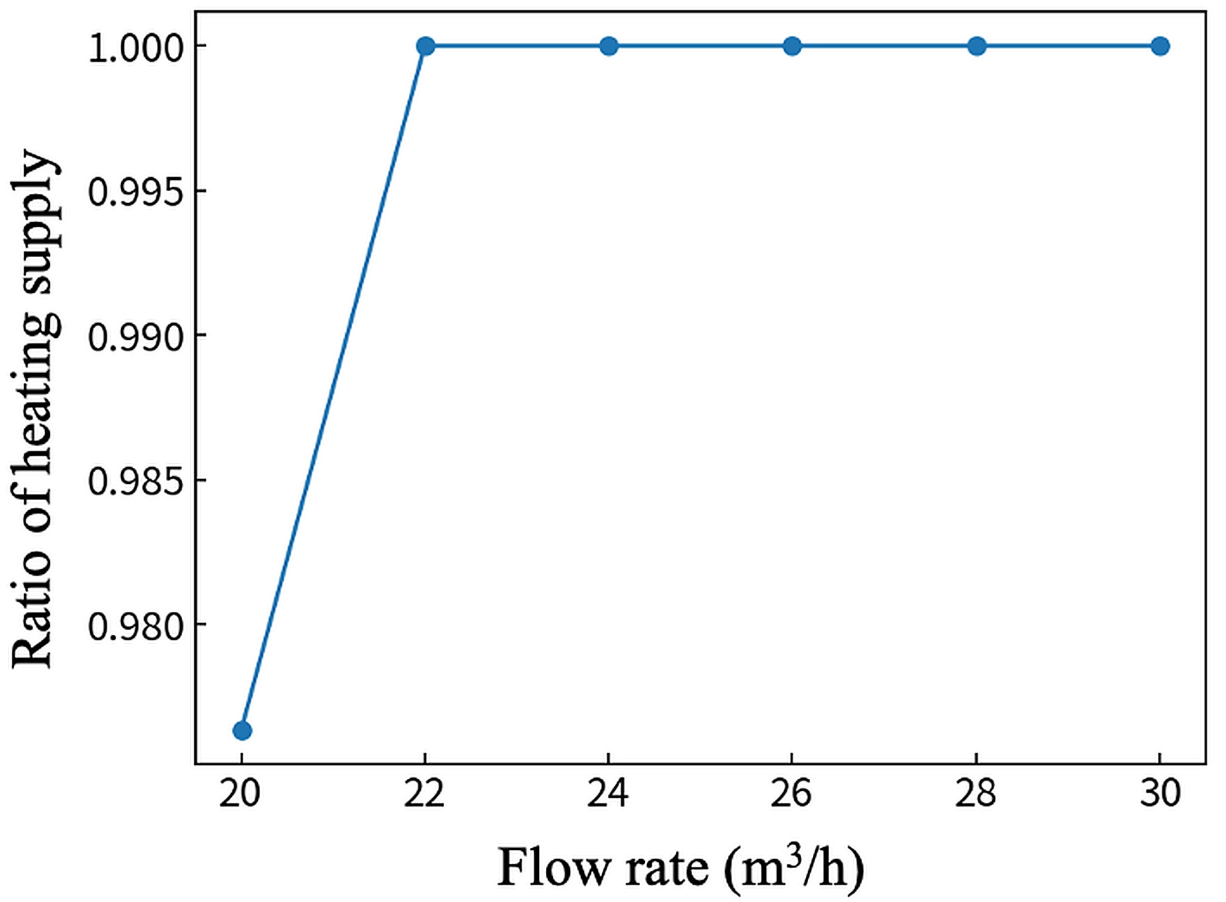
Figure 14. The RHS under different single borehole flow settings. RHS: ratio of heating supply.
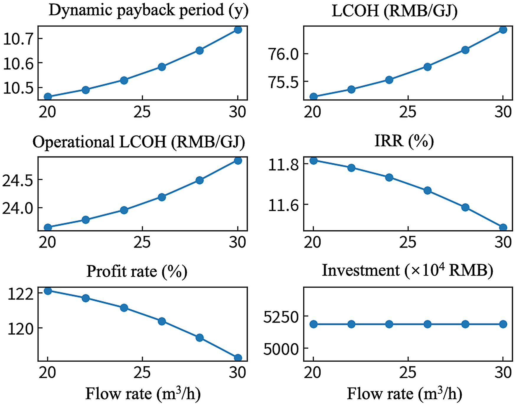
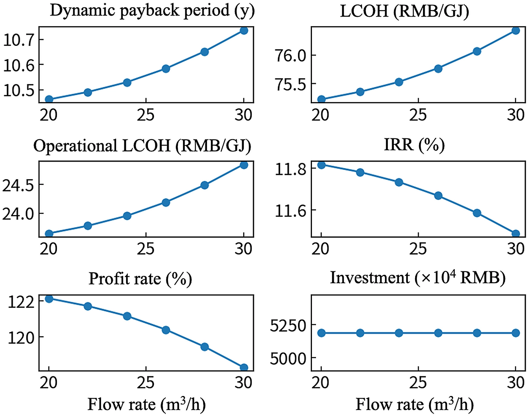
Figure 15. Influence of different single borehole flow on each index. LCOH: levelized cost of heating; IRR: internal rate of return.
3.2.5 Installed capacity ratio of GSHP
By setting different installed capacity ratios of ground-source heat pumps, the variation trends of various economic indicators are calculated. The relevant results are presented in the figure. As the proportion of ground-source heat pump capacity increases, the installed ratio of ASHP decreases correspondingly, with the sum of the two proportions equal to 1. Since the number of drilling wells remains unchanged, the RHS decreases continuously. According to the parametric analysis shown in Figure 16 and Figure 17, the PP, levelized cost, operating cost and initial investment all decline, with distinct differences in the declining rate of each indicator.
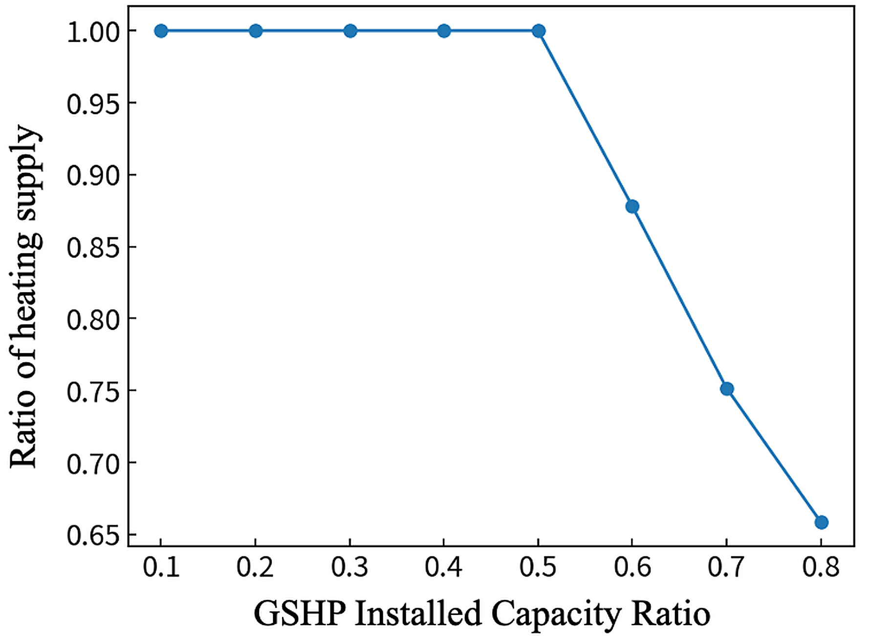
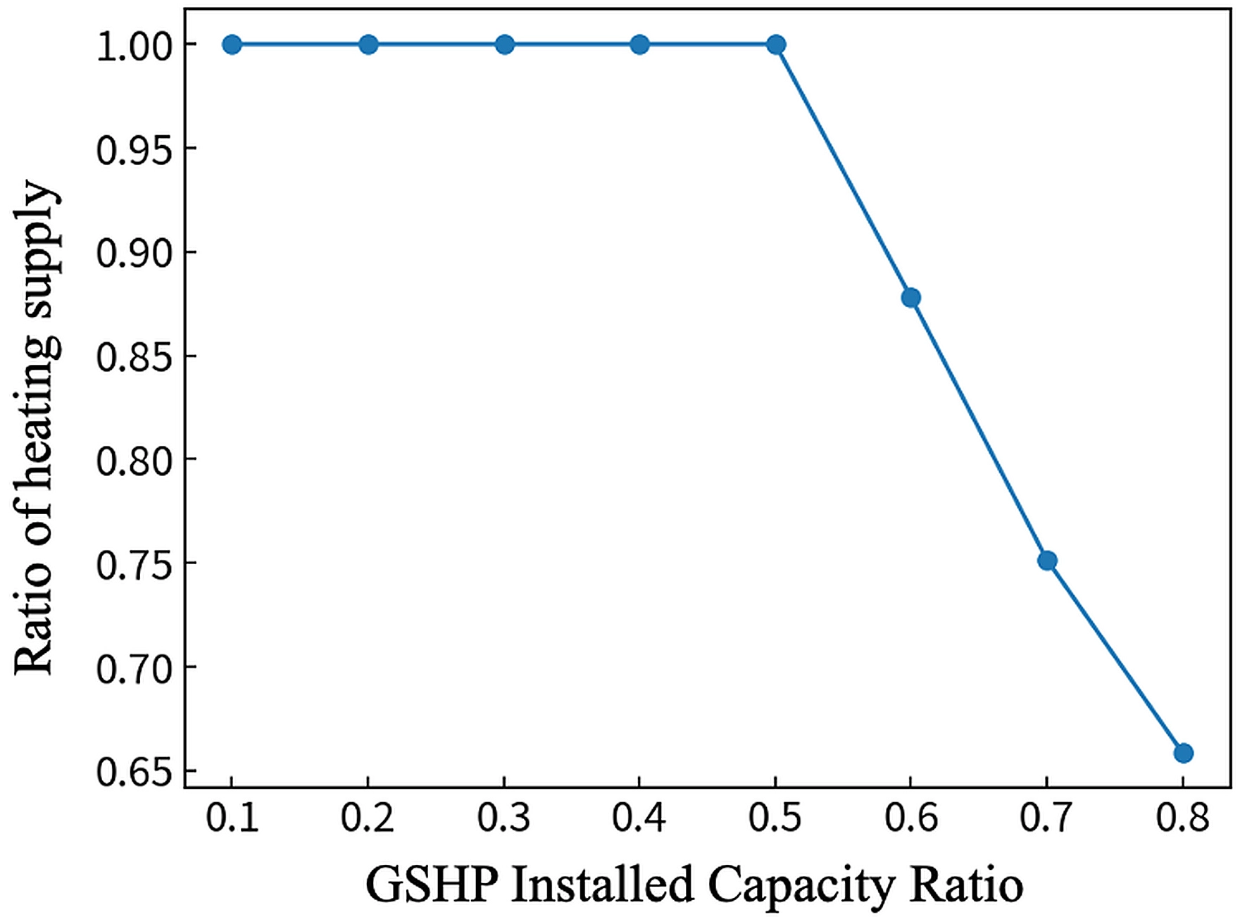
Figure 16. Influence of GSHP installed capacity ratio variation on RHS. GSHP: ground source heat pump; RHS: ratio of heating supply.
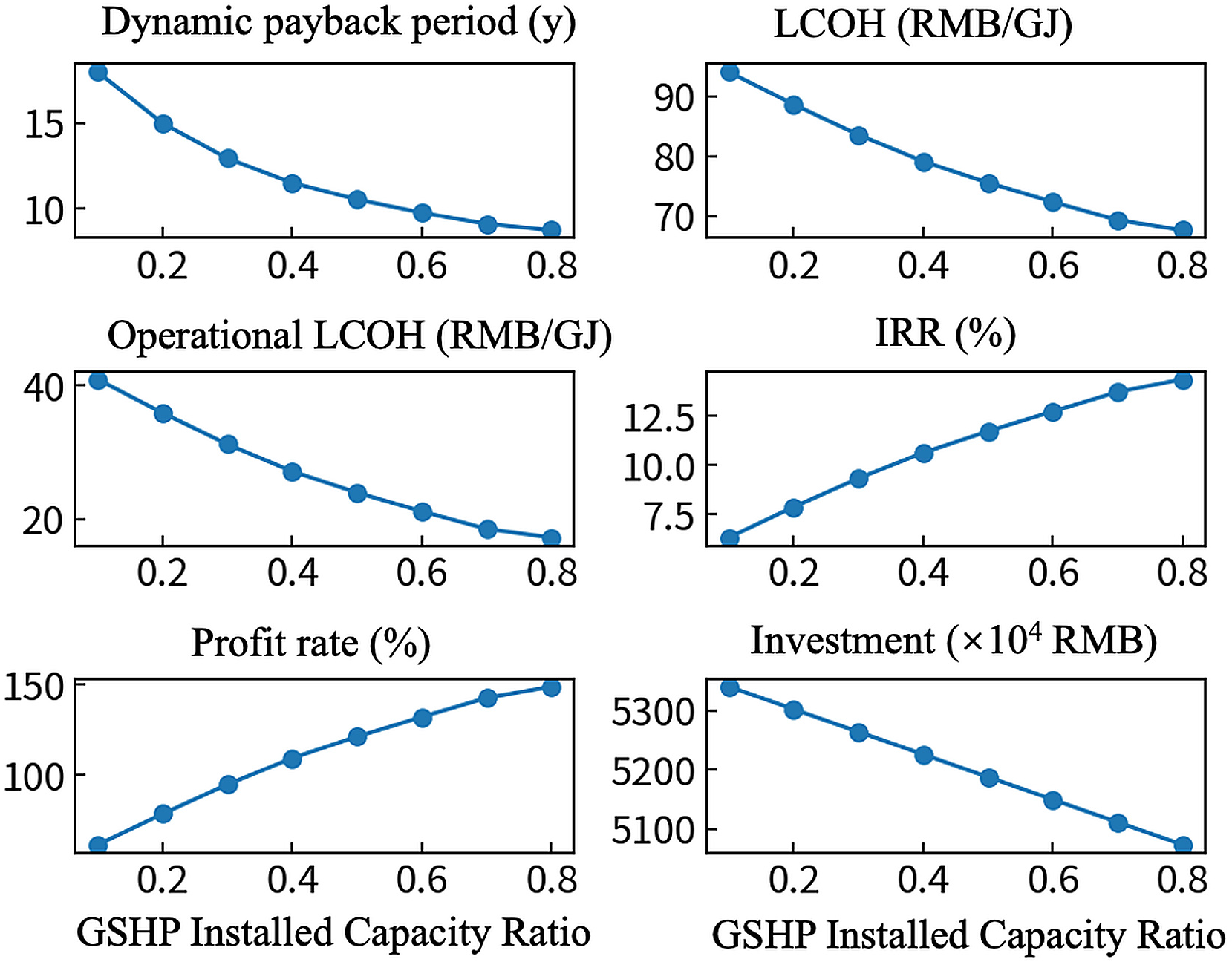
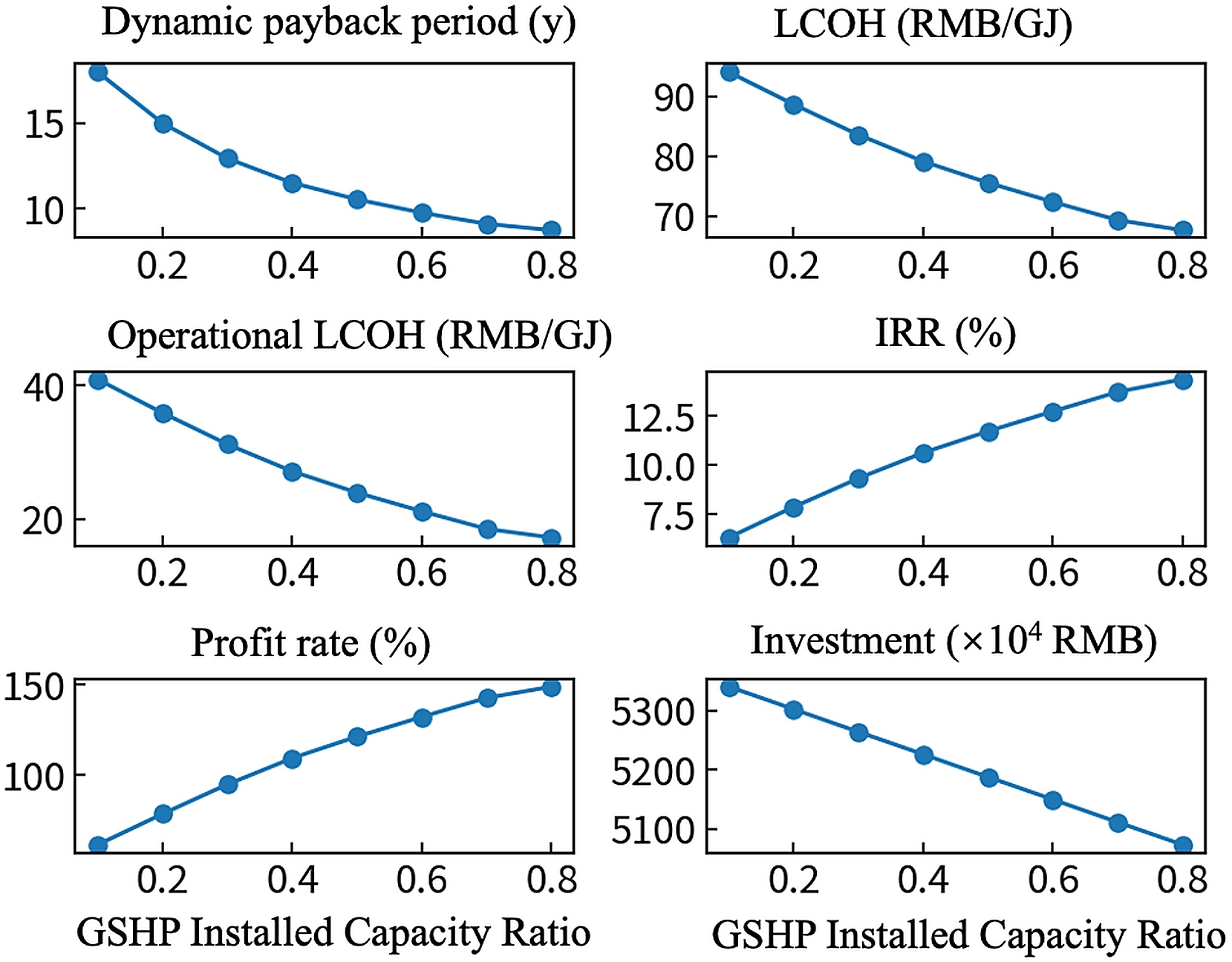
Figure 17. Influence of different GSHP installed capacity ratio on each index. GSHP: ground source heat pump; LCOH: levelized cost of heating; IRR: internal rate of return.
3.2.6 Sensitivity of design parameters to index
By sorting out the above results of parametric analysis, the data in Table 8 can be obtained, which characterizes the sensitivity of each design parameter in terms of its influence degree on economic indicators.
Table 8. Sensitivity analysis of economic index to different design parameters.
| Design Parameter x | Sensitivity Coefficient | |||||
| Payback Period (Year/x) | Levelized Cost (CNY/x) | Levelized Operating Cost (CNY/x) | Internal Rate of Return (%/x) | Profit Margin (%/x) | Initial Investment (10,000 CNY/x) | |
| Number of Boreholes (x = 1) | 1.72 | 3.16 | -0.167 | -1.40 | -12.57 | 373.5 |
| Drilling Depth (x = 100 m) | 0.428 | 0.76 | -0.125 | -0.381 | -3.27 | 99.59 |
| Single Borehole Flow (x = 1 m3/h) | 0.041 | 0.178 | 0.178 | -0.049 | -0.573 | 0.0 |
| GSHP Installed Capacity Ratio (x = 0.1) | -2.99 | -5.42 | -5.02 | 1.55 | 17.13 | -38.12 |
GSHP: ground source heat pump.
For the borehole quantity, each additional borehole in this case increases the PP by 1.72 years and the levelized cost by 3.16 CNY/GJ, while reducing the operating cost by 0.167 CNY/GJ and the profit margin by 12.57%.
For drilling depth, the buried geothermal wells are constructed in a basic unit of 100 meters. The data in the table indicates that every 100-meter growth in drilling depth increases the PP by 0.428 years, the levelized cost by 0.76 CNY/GJ, and decreases the profit margin by 3.27%.
In terms of the operating flow rate of a single borehole, each increase of 1 m3/h in flow rate raises the PP by 0.041 years, increases both levelized cost and operating cost by 0.178 CNY/GJ, and reduces the profit margin by 0.573%.
With regard to the length ratio of the insulation section of the central pipe, every 0.1 increase in the ratio extends the PP by 0.139 years, raises the levelized cost by 0.26 CNY/GJ, and reduces the profit margin by 1.186%.
Finally, the installed capacity ratio of the GSHP unit is analyzed. For every 0.1 increment in this ratio, the PP decreases by 2.99 years, the levelized cost drops by 5.42 CNY/GJ, the operating cost reduces by 5.02 CNY/GJ, and the initial investment decreases by 381,200 CNY.
Accordingly, among all design parameters, the installed capacity ratio of GSHP units and the number of boreholes exert the most significant impacts on evaluation results, followed by the length ratio of the central pipe insulation section and drilling depth. The single borehole flow rate and insulation materials of the central pipe show the weakest influence. This sensitivity analysis provides critical data support for the subsequent Bayesian optimization strategy and calculation.
Based on the sensitivity of the design parameters, they can be categorized into three groups:
Category 1: Installed capacity ratio of cold and heat source equipment, number of boreholes, and drilling depth;
Category 2: Segment length of the central pipe (only applicable when the segmented central pipe design scheme is adopted) and insulation material for the segmented central pipe;
Category 3: Single borehole flow rate.
Therefore, when performing comprehensive system optimization calculations, the sensitivity levels of these three categories can be referenced to conduct step-by-step optimization, thus obtaining optimal design parameters with minimal computational resource consumption.
3.3 Optimization results
3.3.1 Mid-deep geothermal heating system
Calculations were performed with each of the six economic indicators set as an optimization objective, and the corresponding optimization results are presented in Table 9. Except for the objectives of minimizing the levelized operating cost and initial investment, the optimization results for all other indicators are nearly identical. It is noted that minimizing the levelized operating cost converges to a design with 12 geothermal wells, while all other optimizations yield 8 wells. To maintain the RHS of 1, the 8-well schemes adopt a higher water flow rate, whereas minimizing the operating cost tends to select a lower operating flow rate to reduce the pump’s operating power consumption.
Table 9. Optimization of mid-deep geothermal and air-source heat pump combined heating system.
| Different Optimization Objectives | Dynamic Payback Period | Levelized Cost | Levelized Operating Cost | Initial Investment | Internal Rate of Return | Profit Margin |
| Objective | Minimization | Minimization | Minimization | Minimization | Maximization | Maximization |
| Discount Rate | 3% | 3% | 3% | 3% | 3% | 3% |
| GSHP Installed Capacity Ratio | 10% | 39% | 100% | 10% | 10% | 10% |
| Number of Boreholes | 2 | 4 | 11 | 2 | 2 | 2 |
| Drilling Depth | 2,400 | 3,500 | 3,500 | 2,400 | 2,400 | 2,400 |
| Single Borehole Flow | 24 | 24 | 20 | 23 | 23 | 23 |
| Central Pipe Material | Material Fiber-reinforced Polyethylene Insulated Pipe, DN80 | Double-layer Hollow Insulated Steel Pipe | Double-layer Hollow Insulated Steel Pipe | MaterialFiber-reinforced Polyethylene Insulated Pipe, DN80 | MaterialFiber-reinforced Polyethylene Insulated Pipe, DN80 | MaterialFiber-reinforced Polyethylene Insulated Pipe, DN80 |
| Dynamic Payback Period (Year) | 2.37 | 5.69 | 14.67 | 2.37 | 2.37 | 2.37 |
| Static Payback Period (Year) | 2.32 | 5.31 | 12.08 | 2.32 | 2.32 | 2.32 |
| Levelized Cost (CNY/GJ) | 70.68 | 66.30 | 79.30 | 70.68 | 70.68 | 70.68 |
| Levelized Operating Cost (CNY/GJ) | 40.66 | 27.16 | 16.08 | 40.66 | 40.66 | 40.66 |
| Internal Rate of Return (%) | 75.41 | 23.11 | 8.07 | 75.41 | 75.41 | 75.41 |
| Profit Margin (%) | 205.15 | 181.97 | 95.14 | 205.15 | 205.15 | 205.15 |
| Initial Investment (10,000 CNY) | 2,919 | 3,973 | 6,739 | 2,919 | 2,919 | 2,919 |
GSHP: ground source heat pump.
The parameter combinations obtained under different optimization objectives were input into the geothermal system for calculation, yielding the economic indicators listed in Table 10. It can be seen that the optimization results for minimizing the PP, maximizing the IRR, and maximizing the overall profit margin are consistent. Minimizing the operating cost relies primarily on increasing the number of boreholes (regardless of the resulting increase in initial investment) and reducing the operating flow rate as much as possible. The results show that this optimization design is not advisable, as the sole reduction in operating costs leads to other indicators far exceeding their optimal values.
Table 10. Optimization results of mid-deep geothermal standalone heating.
| Different Optimization Objectives | Dynamic Payback Period | Levelized Cost | Levelized Operating Cost | Initial Investment | Internal Rate of Return | Profit Margin |
| Objective | Minimization | Minimization | Minimization | Minimization | Maximization | Maximization |
| Discount Rate | 3% | 3% | 3% | 3% | 3% | 3% |
| Number of Boreholes | 8 | 8 | 12 | 8 | 8 | 8 |
| Drilling Depth | 3,450 | 3,450 | 3,500 | 3,450 | 3,450 | 3,450 |
| Single Borehole Flow | 26 | 26 | 20 | 30 | 26 | 26 |
| Central Pipe Material | Double-layer Hollow Insulated Steel Pipe | Double-layer Hollow Insulated Steel Pipe | Double-layer Hollow Insulated Steel Pipe | Fiber-reinforced Polyethylene Insulated Pipe, DN75 | Double-layer Hollow Insulated Steel Pipe | Double-layer Hollow Insulated Steel Pipe |
| Dynamic Payback Period (Year) | 9.05 | 9.05 | 16.80 | 9.18 | 9.05 | 9.05 |
| Static Payback Period (Year) | 8.06 | 8.06 | 13.43 | 8.16 | 8.06 | 8.06 |
| Levelized Cost (CNY/GJ) | 67.34 | 67.34 | 83.64 | 69.20 | 67.34 | 67.34 |
| Levelized Operating Cost (CNY/GJ) | 17.55 | 17.55 | 16.11 | 20.15 | 17.55 | 17.55 |
| Internal Rate of Return (%) | 13.83 | 13.83 | 6.86 | 13.61 | 13.83 | 13.83 |
| Profit Margin (%) | 146.55 | 146.55 | 82.03 | 142.10 | 146.55 | 146.55 |
| Initial Investment (10,000 CNY) | 5,235 | 5,235 | 7,222 | 5,152 | 5,235 | 5,235 |
3.3.2 Mid-deep geothermal and air-source heat pump combined heating system
For the configuration of mid-deep geothermal combined with air-source heat pump in a residential heating project in Xi’an, taking a discount rate of 3% as an example, and without considering the annual variation in occupancy rate or the segmented design of the central pipe, optimization design calculations of the geothermal system were carried out. Multiple economic indicators, including dynamic PP, static PP, and levelized cost, were used as optimization objectives. The optimization results under different optimization objectives were examined and compared.
The calculation results are presented in Table 9. The optimal parameter configurations obtained when taking dynamic PP, IRR, and profit margin as optimization objectives are identical, indicating that these three economic indicators share the same optimization orientation in this case. When the levelized cost over the whole life cycle is taken as the optimization objective, the obtained GSHP installed capacity ratio is closest to that selected in practical engineering applications. This approach is consistent with the optimization design concept that considers the total life-cycle cost, with the only difference being that the cost is normalized by the user-side heating load.
When minimizing the levelized operating cost is set as the optimization objective, the algorithm automatically selects a 100% share of the GSHP system, as its COP is much higher than that of the ASHP system. When the optimization objective is minimizing the initial investment, the algorithm tends to minimize the installed capacity ratio of the GSHP system.
Overall, under the influence of the discount rate, the optimization design results tend to favor parameter combinations that reduce the initial investment and enable faster payback of the upfront costs. In contrast, using the levelized cost over the whole life cycle as the optimization indicator allows for a more comprehensive consideration of the system’s subsequent operating costs.
3.3.3 Mid-deep geothermal and gas boiler combined heating system
For the configuration of mid-deep geothermal combined with gas-fired boilers in a residential heating project in Xi’an, taking a discount rate of 3% as an example, and without considering the annual variation in occupancy rate or the segmented design of the central pipe, optimization design calculations of the geothermal system were carried out with multiple economic indicators, including dynamic PP, static PP, and levelized cost, as optimization objectives. The optimization results under different optimization objectives were examined and compared.
The calculation results are presented in Table 11. In this case, several optimization cases yield relatively short PPs, mainly because the gas-fired boiler system has a lower initial investment. Therefore, under the optimization orientation of indicators such as PP, initial investment, and IRR, the algorithm tends to select a lower installed capacity ratio of the GSHP system. When minimizing the levelized operating cost is set as the optimization objective, the optimization result is consistent with that of the previous mid-deep geothermal + air-source heat pump system, where the algorithm automatically selects a 100% share of the GSHP system. When taking levelized cost and profit margin as optimization objectives, the obtained capacity ratio is most consistent with that adopted in practical engineering applications: a 49% installed capacity ratio for the GSHP system and 51% for the gas-fired boiler system, a drilling depth set to the maximum searched value of 3,500 m, and the double-layer hollow insulated steel pipe with the best thermal insulation performance selected as the central pipe material.
Table 11. Optimization of mid-deep geothermal and gas-fired boiler combined heating system.
| Different Optimization Objectives | Dynamic Payback Period | Levelized Cost | Levelized Operating Cost | Initial Investment | Internal Rate of Return | Profit Margin |
| Objective | Minimization | Minimization | Minimization | Minimization | Maximization | Maximization |
| Discount Rate | 3% | 3% | 3% | 3% | 3% | 3% |
| GSHP Installed Capacity Ratio | 10% | 49% | 100% | 10% | 10% | 49% |
| Number of Boreholes | 2 | 5 | 11 | 2 | 2 | 5 |
| Drilling Depth | 2,400 | 3,500 | 3,500 | 2,400 | 2,400 | 3,500 |
| Single Borehole Flow | 23 | 23 | 20 | 23 | 23 | 23 |
| Central Pipe Material | Fiber-reinforced Polyethylene Insulated Pipe, DN80 | Double-layer Hollow Insulated Steel Pipe | Double-layer Hollow Insulated Steel Pipe | Fiber-reinforced Polyethylene Insulated Pipe, DN80 | Fiber-reinforced Polyethylene Insulated Pipe, DN80 | Double-layer Hollow Insulated Steel Pipe |
| Dynamic Payback Period (Year) | 2.35 | 6.79 | 14.67 | 2.35 | 2.35 | 6.79 |
| Static Payback Period (Year) | 2.30 | 6.24 | 12.08 | 2.30 | 2.30 | 6.24 |
| Levelized Cost (CNY/GJ) | 80.46 | 68.16 | 79.30 | 80.46 | 80.46 | 68.16 |
| Levelized Operating Cost (CNY/GJ) | 50.56 | 25.79 | 16.08 | 50.56 | 50.56 | 25.79 |
| Internal Rate of Return (%) | 76.73 | 18.95 | 8.07 | 76.73 | 76.73 | 18.95 |
| Profit Margin (%) | 154.78 | 165.39 | 95.1 | 154.78 | 154.78 | 165.39 |
| Initial Investment (10,000 CNY) | 2,772 | 4,272 | 6,739 | 2,772 | 2,772 | 4,272 |
GSHP: ground source heat pump.
3.3.4 Operational carbon-emission comparison of hybrid geothermal systems
To compare the operational carbon-emission performance of the three systems, annual emissions were calculated based on the method described in Figure 7. The results are list in Table 12. The system configurations used in carbon emission calculation are from levelized cost optimization. It is clear that the geothermal standalone system reaches the highest potential of carbon emission reduction. In contrast, the hybrid system of geothermal and air-source heat pump saves the least carbon emission because the system optimization goal is levelized cost of the entire operation period.
Table 12. Annual operational carbon emissions of hybrid geothermal systems.
| Different hybrid geothermal system | Geothermal standalone | Geothermal and air-source heat pump | Geothermal and gas boiler |
| System configurations | Configurations based on levelized cost optimization | ||
| Ratio of ground source heat pump | 100% | 39% | 49% |
| Ratio of other heating cooling sources | 0% | 61% | 51% |
| Carbon emission benchmark (tCO2/year) | 2,240.1 | 2,240.1 | 2,240.1 |
| Carbon emission of geothermal system (tCO2/year) | 1,055.0 | 1,632.7 | 1,322.8 |
| Carbon emission reduction (tCO2/year) | 1,185.1 | 607.3 | 917.3 |
3.4 Discussions
Our results demonstrate that incorporating long-term thermal attenuation and user-side load uncertainty into the techno-economic optimization substantially alters the optimal design of hybrid geothermal systems. Unlike conventional life-cycle economic assessments that assume constant thermal performance throughout the project lifetime, the proposed framework captures the gradual degradation of borehole thermal performance, resulting in longer PPs and different optimal design configurations. This finding is consistent with previous studies showing that long-term subsurface thermal interactions significantly influence the economic viability of geothermal systems and should not be neglected during system design[32]. Furthermore, the sensitivity analysis indicates that the installed capacity ratio of the GSHP and the number of boreholes are the dominant design variables, whereas borehole flow rate has a comparatively limited influence. Similar conclusions have been reported by Lund et al.[33] and Self et al.[34], who emphasized that appropriate sizing of ground heat exchangers has a greater impact on overall system economics than operational parameter adjustment.
Compared with previous geothermal techno-economic studies, which primarily focused on either thermodynamic optimization or simplified economic evaluation (e.g., the study[17]), the proposed framework integrates a detailed borehole heat transfer model, life-cycle economic assessment, uncertainty analysis, and Bayesian optimization into a unified workflow. This enables the optimization process to account for both transient thermal behavior and long-term economic performance while maintaining acceptable computational efficiency. Although the case study is based on residential heating in Xi’an, the framework is not restricted to a specific geological condition or auxiliary heating technology. By updating regional geological properties, load profiles, energy prices, and policy incentives, the methodology can be readily extended to other geothermal heating scenarios or hybrid renewable energy systems. Therefore, the proposed framework provides a practical decision-support tool for improving the robustness and economic competitiveness of geothermal projects under realistic operating conditions.
4. Conclusions
This study establishes a comprehensive economic analysis model for geothermal systems and for heating and cooling systems coupled with auxiliary cold and heat sources. The model can calculate equipment capacities, initial investment, maintenance cost, operating cost, system revenue, and other cost or revenue items, while comprehensively considering relevant influencing factors for each item. On this basis, the model can rapidly calculate multiple economic indicators for geothermal heating and cooling systems and evaluate such systems from multiple perspectives over the entire life-cycle.
Based on the proposed life-cycle analysis and optimization framework for hybrid geothermal systems, a series of investigations were conducted to analyze both non-design and design parameters of geothermal systems. The main conclusions are summarized as follows:
1. The decline in fluid temperature during the long-term operation of geothermal borehole systems has an important impact on system economic performance. Numerical simulations reveal that a 2 °C decline in fluid temperature increases the PP by approximately 0.3 years. In addition, the user-side heating load may deviate from the design value. When the deviation ratio is 10%, the PP may be overestimated or underestimated by about 2 years; when the deviation ratio is 20%, the difference can reach approximately 5 years at most.
2. The influences of borehole number, drilling depth, borehole flow rate, and installed capacity of the ground-source heat pump on various economic indicators are analyzed. Moreover, the sensitivities of these design parameters to the economic indicators are determined. Among all design parameters, the installed capacity ratio of GSHP units and the number of boreholes exert the most significant impacts on the evaluation results. This sensitivity analysis provides important data support for the subsequent Bayesian optimization strategy and calculations.
3. Optimizations are conducted for three different types of geothermal systems. The optimization results for minimizing the PP, maximizing the IRR, and maximizing the overall profit margin are consistent. Minimizing operating cost relies primarily on increasing the number of boreholes, regardless of the resulting increase in initial investment, and reducing the operating flow rate as much as possible. This optimization design is not advisable, because reducing operating costs alone causes other indicators to deviate substantially from their optimal values. By contrast, the combined system of ground-source heat pump and gas boiler can achieve a much shorter PP than the standalone ground-source heat pump system.
Future research can further extend the proposed life-cycle analysis and optimization framework in several aspects. First, the current framework can be coupled with a more detailed life-cycle carbon-emission model to simultaneously evaluate economic performance, energy efficiency, and carbon-reduction benefits. Second, although this study considers long-term thermal attenuation and user-side load fluctuation, more comprehensive uncertainty analysis should be conducted by incorporating variations in geothermal conditions, energy prices, equipment performance degradation, and policy incentives. Third, the framework should be validated using additional engineering projects in different climatic zones, building types, and geological conditions to improve its general applicability. In addition, future studies may integrate real-time monitoring data and intelligent control strategies into the optimization process, enabling adaptive operation of hybrid geothermal systems under dynamic load conditions. Finally, multi-objective optimization considering economic cost, carbon emissions, thermal reliability, and system resilience should be further developed to support the design of low-carbon and high-performance geothermal energy systems for buildings.
Authors contribution
Wang W: Writing-original draft, methodology, formal analysis, project administration.
Cheng H: Writing-original draft, methodology, formal analysis.
Wen J: Writing-review & editing, supervision.
Wang X: Investigation, resources.
Yin K: Methodology, software.
Liu L: Formal analysis, software.
Wang X: Writing-review & editing, supervision.
Luo Y: Conceptualization, methodology.
Conflicts of interest
Wentan Wang, Jiangtao Wen, Xi Wang, Kui Yin, Li Liu, and Xin Wang are employees of the China Construction Third Engineering Bureau Group Co., Ltd. The other authors declare no conflicts of interest.
Ethical approval
Not applicable.
Consent to participate
Not applicable.
Consent for publication
Not applicable.
Availability of data and materials
Data supporting the findings of this study are available from the corresponding author upon reasonable request.
Funding
This work was supported by the CCTEB Institute of Green and Low Carbon Technology (Grant No. DTY-2025-01).
Copyright
© The Author(s) 2026.
References
-
1. Jacobson MZ, Sambor DJ, Fan YF, Mühlbauer A, DiBari GC. The impact of enhanced geothermal systems on transitioning all energy sectors in 150 countries to 100% clean, renewable energy. Cell Rep Sustain. 2026;3(2):100611.[DOI]
-
2. Boretti A. Enhanced geothermal systems: Potential, challenges, and a realistic path to integration in a sustainable energy future. Next Energy. 2025;8:100332.[DOI]
-
3. Xia ZH, Jia GS, Ma ZD, Wang JW, Zhang YP, Jin LW, et al. Analysis of economy, thermal efficiency and environmental impact of geothermal heating system based on life cycle assessments. Appl Energy. 2021;303:117671.[DOI]
-
5. Compernolle T, Welkenhuysen K, Petitclerc E, Maes D, Piessens K. The impact of policy measures on profitability and risk in geothermal energy investments. Energy Econ. 2019;84:104524.[DOI]
-
6. Ge Z, Fu Y, Li J, Xiong X, Bai X, Song G, et al. Tri-objective optimization and comprehensive performance evaluation of geothermal-driven transcritical organic Rankine cycle. Appl Therm Eng. 2026;285:129221.[DOI]
-
7. Schifflechner C, Dawo F, Eyerer S, Wieland C, Spliethoff H. Thermodynamic comparison of direct supercritical CO2 and indirect brine-ORC concepts for geothermal combined heat and power generation. Renew Energy. 2020;161:1292-1302.[DOI]
-
8. Shoeibi Omrani P, Egberts PJP, Rijnaarts HHM, Shariat Torbaghan S. Geothermal plant operation and control under demand uncertainties. Renew Energy. 2026;257:124805.[DOI]
-
9. Guo X, Abed AM, Alghassab MA, Alhomayani FM, Mahariq I, Elmasry Y, et al. Development of a geothermal-driven multi-output scheme for electricity, cooling, and hydrogen production: Techno-economic assessment and genetic algorithm-based optimization. Case Stud Therm Eng. 2024;63:105228.[DOI]
-
10. Chen G, Jiao JJ, Liu Q, Wang Z, Jin Y. Machine-learning-accelerated multi-objective design of fractured geothermal systems. Nexus. 2024;1(4):100044.[DOI]
-
11. Karlsdottir MR, Heinonen J, Palsson H, Palsson OP. Life cycle assessment of a geothermal combined heat and power plant based on high temperature utilization. Geothermics. 2020;84:101727.[DOI]
-
12. Violante AC, Donato F, Guidi G, Proposito M. Comparative life cycle assessment of the ground source heat pump vs air source heat pump. Renew Energy. 2022;188:1029-1037.[DOI]
-
13. Hai T, Zhou J, Almashhadani YS, Chaturvedi R, Alshahri AH, Almujibah HR, et al. Thermo-economic and environmental assessment of a combined cycle fueled by MSW and geothermal hybrid energies. Process Saf Environ Prot. 2023;176:260-270.[DOI]
-
14. Li J, Tarpani RRZ, Stamford L, Gallego-Schmid A. Life cycle sustainability assessment and circularity of geothermal power plants. Sustain Prod Consum. 2023;35:141-156.[DOI]
-
15. Frick S, Kaltschmitt M, Schröder G. Life cycle assessment of geothermal binary power plants using enhanced low-temperature reservoirs. Energy. 2010;35(5):2281-2294.[DOI]
-
16. Lacirignola M, Blanc I. Environmental analysis of practical design options for enhanced geothermal systems (EGS) through life-cycle assessment. Renew Energy. 2013;50:901-914.[DOI]
-
17. Gerber L, Maréchal F. Environomic optimal configurations of geothermal energy conversion systems: Application to the future construction of Enhanced Geothermal Systems in Switzerland. Energy. 2012;45(1):908-923.[DOI]
-
18. Wang Y, Du Y, Wang J, Zhao J, Deng S, Yin H, et al. Comparative life cycle assessment of geothermal power generation systems in China. Resour Conserv Recycl. 2020;155:104670.[DOI]
-
19. Xia Z, Jia G, Tao Z, Jia W, Shi Y, Jin L, et al. Multi-objective optimization of geothermal heating systems based on thermal economy and environmental impact evaluation. Renew Energy. 2024;237:121858.[DOI]
-
20. Turner I, Bamber N, Andrews J, Pelletier N. Systematic review of the life cycle optimization literature, and recommendations for performance of life cycle optimization studies. Renew Sustain Energy Rev. 2025;208:115058.[DOI]
-
21. Dong S, Yu Y, Wang H, Yao Y, Ni L. An economic-energetic-environmental evaluation algorithm for hybrid mid-depth geothermal heating system. Energy. 2023;282:128903.[DOI]
-
22. Fan Y, Fan Y, Li M, Shi H, Zhou P. Optimizing operational strategy for medium-depth hydrothermal geothermal cascade heating system. Appl Therm Eng. 2026;296:130768.[DOI]
-
23. Luo Y, Shen J, Song Y, Tian Z, Fan J, Zhang L, et al. A unified analytical model for vertical ground heat exchangers: Non-uniform finite line source method (NFLS). Renew Energy. 2026;256:124072.[DOI]
-
24. Luo Y, Cheng N, Xu G. Analytical modeling and thermal analysis of deep coaxial borehole heat exchanger with stratified-seepage-segmented finite line source method (S3-FLS). Energy Build. 2022;257:111795.[DOI]
-
25. Luo Y, Guo H, Meggers F, Zhang L. Deep coaxial borehole heat exchanger: Analytical modeling and thermal analysis. Energy. 2019;185:1298-1313.[DOI]
-
26. Cai W, Wang F, Chen S, Chen C, Liu J, Deng J, et al. Analysis of heat extraction performance and long-term sustainability for multiple deep borehole heat exchanger array: A project-based study. Appl Energy. 2021;289:116590.[DOI]
-
27. Zhang L, Zhou M, Yang C, Li Y, Fu Z, Wang J, et al. Evaluation and optimization of water source heat pump for district heating: A case study in steel plant. Int J Energy Res. 2020;44(12):9399-9413.[DOI]
-
28. Li C, Mao J, Zhang H, Xing Z, Li Y, Zhou J, et al. Numerical simulation of horizontal spiral-coil ground source heat pump system: Sensitivity analysis and operation characteristics. Appl Therm Eng. 2017;110:424-435.[DOI]
-
29. Abouzied AS, Basem A, Shaban M, Alhomayani FM, Dutta AK, Abduvalieva D, et al. A geothermal-based freshwater/cooling system assisted by heat recovery sections: 3E analysis and techno-economic optimization using genetic algorithm. Case Stud Therm Eng. 2024;63:105267.[DOI]
-
30. Liu Z, Gudala M, Katterbauer K, Yan B. Robust optimization of fully coupled geothermal reservoir and power plant system based on deep learning. Energy Convers Manag: X. 2026;30:101556.[DOI]
-
31. Zhang Z, Jia G, Ma Z, Hao J, Zhang M, Cao Y, et al. Parameter optimization and ground temperature analysis of a solar-assisted medium-deep geothermal heating system under long-term operation. Renew Energy. 2026;261:125234.[DOI]
-
32. Eskilson P. Thermal analysis of heat extraction boreholes [dissertation]. Lund: Lund Institute of Technology; 1987. Available from: https://www.osti.gov/etdeweb/biblio/7778302
-
33. Lund JW, Freeston DH, Boyd TL. Direct utilization of geothermal energy 2010 worldwide review. Geothermics. 2011;40(3):159-180.[DOI]
-
34. Self SJ, Reddy BV, Rosen MA. Geothermal heat pump systems: Status review and comparison with other heating options. Appl Energy. 2013;101:341-348.[DOI]
Copyright
© The Author(s) 2026. This is an Open Access article licensed under a Creative Commons Attribution 4.0 International License (https://creativecommons.org/licenses/by/4.0/), which permits unrestricted use, sharing, adaptation, distribution and reproduction in any medium or format, for any purpose, even commercially, as long as you give appropriate credit to the original author(s) and the source, provide a link to the Creative Commons license, and indicate if changes were made.
Publisher’s Note
Science Exploration remains a neutral stance on jurisdictional claims in published
maps
and institutional affiliations. The views expressed in this article are solely those
of
the author(s) and do not reflect the opinions of the Editors or the publisher.
Share And Cite


Science Exploration Style
Wang W, Cheng H, Wen J, Wang X, Yin K, Liu L, et al. Life cycle techno-economic analysis and optimization framework of hybrid deep ground source heat pump system for low carbon buildings. J Build Des Environ. 2026;4:202621. https://doi.org/10.70401/jbde.2026.0041
Tips
Copy completed.
Submit a Manuscript
Author Instructions
Cite this Article
Article Metrics
0
View
0
Download
Cited
Article Updates

 Get citation
Science Exploration Style

Wang W, Cheng H, Wen J, Wang X, Yin K, Liu L, et al. Life cycle techno-economic analysis and optimization framework of hybrid deep ground source heat pump system for low carbon buildings. J Build Des Environ. 2026;4:202621. https://doi.org/10.70401/jbde.2026.0041
copy
Share Link
copy
Subscribe