1. Introduction

Thermal conductivity and thermal diffusivity are two fundamental properties that govern a material’s steady-state and transient response under thermal loading. Accurate measurement of these properties is of great significance and is influenced by multiple factors, including the sample’s physical characteristics, ambient temperature, and inherent thermal conductivity or diffusivity. Although it is technically feasible to determine thermal conductivity using steady-state methods, by applying a constant heat flux and measuring the resulting temperature gradient, such approaches are often laborious and require precise control of heating and boundary conditions^[1,2]. In contrast, transient techniques, which capture a material’s response in the time or frequency domain under pulsed or periodic thermal excitation, offer a more straightforward and efficient solution. These methods enable rapid and reliable determination of thermal conductivity and thermal diffusivity. Representative examples include the transient hot-wire method, regarded as the gold standard for liquids and powders^[3,4], and the laser flash technique, widely employed for solids^[5]. Other notable techniques include the 3ω method and time or frequency-domain pump-probe approaches for measuring thermal conductivity and interfacial thermal resistance in coatings^[6-8]. A key driver in the evolution of these measurement techniques is the size and geometry of the material. Recent breakthroughs in micro- and nanoscale fabrication, particularly for two-dimensional (2D) structures such as films and coatings and one-dimensional (1D) architectures such as wires and fibers, have created an urgent need for advanced thermal characterization tools that can elucidate underlying structure–property relationships. For clarity, “1D materials” refers to truly one-dimensional structures such as wires and fibers, where heat conduction is effectively confined to a single spatial dimension. Conversely, certain suspended films and ultrathin coatings, although structurally 2D, may exhibit quasi-1D heat conduction behavior when lateral thermal transport is restricted by geometry or boundary conditions. Under Transient Electro-Thermal (TET) measurement conditions, these cases are often modeled using 1D approximations. Liu et al.^[6] provide a broad discussion of such developments in photon-excitation-based techniques. A fundamental priority in developing thermal conductivity and thermal diffusivity measurement methods is simplicity, which encompasses simplicity in physical principles, experimental implementation, and data reduction. This simplicity is crucial for minimizing uncertainty, ensuring data accuracy, and improving measurement throughput.

Electro-thermal methods, such as the suspended micro-bridge technique, the 3ω method, electron-beam self-heating, and the T-bridge method, determine a material’s thermal conductivity by analyzing changes in its thermal resistance with temperature. Among these, the transient plane source (TPS) method, also known as the hot disk technique, is widely used for measuring the thermal conductivity and diffusivity of a broad range of materials, including thin films, bulk solids, pastes, adhesives, liquids, gels, and powders. The TPS method employs a disk-shaped nickel sensor insulated by thin dielectric layers, which serves as both the heat source and the thermometer, and is typically positioned between two pieces of the sample. This technique is valued for its rapid, convenient, and versatile measurements, as it extracts thermal transport properties from the sensor’s time-dependent temperature response^[9,10]. However, the accuracy of the TPS method can be compromised by several factors, including thermal contact resistance (TCR) at the sample interfaces, the finite thickness and thermal mass of the sensor’s insulation, and the geometry of the sensor itself. These limitations are particularly significant when characterizing thin films and low-conductivity materials^[9,11]. To overcome these challenges, several enhancements have been proposed: (1) Use of a background slab to confine heat flow to one dimension and decouple the sensor’s TCR from the film’s thermal resistance, combined with multi-thickness measurements and linear regression for more accurate property extraction^[11]. (2) Development of analytical and numerical correction models, such as polynomial correction functions, which reduce measurement inaccuracies from up to 40% to less than 4% in low-conductivity samples^[9]. (3) Advancement of theoretical modeling and data analysis, including realistic sensor and multilayer models, derivative-based analysis, and sophisticated regression and sensitivity techniques. These improvements collectively reduce fitting errors for high-conductivity materials from nearly 97% to within 10%, and enable accurate measurements on smaller samples with shorter test durations^[12]. In addition, photothermal techniques offer powerful, non-contact, high-resolution capabilities for microscale thermal transport studies. For example, the recently developed Three-Dimensional Spatially Resolved Lock-In Micro-Thermography method employs a fully optical configuration with micrometer-scale spatial resolution to determine the complete 3D anisotropic thermal conductivity tensor. This approach overcomes the limitations of conventional vector-based or two-dimensional methods by directly mapping phase and amplitude responses from three orthogonal surfaces, thereby enabling high-throughput measurements even for samples with significant surface roughness^[13].

The suspended micro-bridge and T-bridge methods are classical approaches for characterizing 1D materials; however, they often require complex microfabrication, involve significant challenges in evaluating contact resistance, and offer limited scalability. The 3ω method, while widely used for thin films and capable of extracting both in-plane and cross-plane properties, is applicable only to electrically conductive films and becomes less suitable for few-layer 2D materials. Time-domain thermoreflectance (TDTR) and Raman-based techniques are powerful tools for probing nanoscale heat transport, but they require highly sophisticated setups, surface modifications such as metal coating, and often face difficulties in the absolute quantification of absorbed laser power or in application to metallic or centrosymmetric materials. A comparative summary of these methods is presented in Table 1. In this review, we provide an in-depth discussion of the TET technique, developed by Wang’s group, for measuring the thermal diffusivity and conductivity of 1D and 2D materials, including thin films and fibers/wires^[14]. The paper addresses the physical principles of TET operation, the underlying physical and mathematical models for data reduction, measurement repeatability and accuracy, and the extension of TET for characterizing materials down to atomic-scale thickness. In addition, we review the application of TET for in-situ dynamic thermal property measurements during structural evolution and the implementation of the zero-temperature-rise method for ultimate accuracy. Finally, we provide an outlook on future developments and potential applications of this technique.

2. Physics and Theory of the TET Technique

2.1 Foundational theory

The TET technique, first developed by our group in 2007, provides highly accurate measurements of the thermal diffusivity (α) of fiber-like and thin-film materials^[14-21]. This range of materials includes polyacrylonitrile (PAN) wires^[22], carbon nanocoils^[23], 3C crystalline silicon carbide (SiC) microwires^[24], carbon nanotubes^[25], gas diffusion layers of PEM fuel cells^[26], polypropylene separator^[17], and others. In this technique, the sample is suspended over a trench and bonded to two aluminum electrodes using silver paste, ensuring strong electrical and thermal contacts. As illustrated in Figure 1a, during TET measurement, a step DC current (I) is applied to the sample, generating Joule heating and causing its temperature (T) to rise, which in turn changes its resistance (R). This resistance change results in a transient variation in the measured voltage (V). The heating duration is selected to allow the sample to reach a steady-state temperature, while sufficient cooling time between current pulses prevents thermal accumulation from previous cycles. The voltage-time (V-t) response, reflecting the sample’s thermal behavior, is then analyzed to extract its effective thermal diffusivity (α_eff). It should be noted that α_eff may include contributions from radiation and thin conductive coatings (applied to nonconductive samples), which can be accounted for and excluded later. Due to the sample’s large aspect ratio (length to thickness), heat conduction is effectively one-dimensional along its length (L). Moreover, all measurements are conducted under vacuum conditions (< 0.2 mTorr) to suppress convective heat transfer. The transient heat conduction along the sample’s length (x-axis) is described by the following equation^[14]:

Display Full Size

Figure 1. Physics and theory of the TET technique. (a) The schematic of the experimental set-up^[27]; (b) The normalized temperature rise of a Pt wire during TET characterization, along with results from three different data analysis techniques^[14]. TET: Transient Electro-Thermal.

(1)$\frac{\partial \left(T\rho c_p\right)}{\partial t}=\frac{\partial }{\partial x}\left(k\frac{\partial T}{\partial x}\right)+{\dot{q}}_0$

Here, ρ, c_p, and k represent the density, specific heat capacity, and thermal conductivity of the sample, respectively. The term ${\dot{q}}_0$ (in W/m³) corresponds to the volumetric heat generation induced by the electrical current. Given the overall setup, the initial condition is defined as T(x, t = 0) = T_0, where T₀ is the ambient temperature. Since the aluminum electrodes can be regarded as ideal heat sinks, the boundary conditions are T(x = 0, t) = T(x = L, t) = T₀. By solving Eq. (1) using the Green’s function integral method, the temperature distribution along the sample length can be obtained as ^[14]:

(2)$T(x,t)=T_0+\frac{\alpha }{k}{\int }_{\tau =0}^t{\int }_{x^{\prime }=0}^L{q}_0{G}_{X11}d{x}^{\prime }d\tau$

where G_X11 denotes the Green’s function:

(3)$G_{X11}(x,t\mid x^{\prime },\tau )=\frac{2}{L}\sum _{m=1}^{\infty }\exp [-m^2{\pi }^2{\alpha }_{eff}(t-\tau \left)/L^2\right]\times \sin \left(m\pi \frac{x}{L}\right)\sin \left(m\pi \frac{x^{\prime }}{L}\right)$

The average temperature of the sample is determined by integration as follows^[14]:

(4)$T\left(t\right)=\frac{1}{L}{\int }_{x=0}^{L}T(x,t)dx=T_0+\frac{8q_0{L}^2}{k{\pi }^4}\sum _{m=1}^{\infty }\frac{1-\exp [-(2m-1{)}^2{\pi }^2{\alpha }_{eff}t/L^2]}{(2m-1{)}^4}$

As time approaches infinity (t→∞), the temperature distribution reaches steady state. The final steady-state average temperature of the wire is:

(5)$T(t\to \infty )=T_0+\frac{{\dot{q}}_0{L}^2}{12k}$

The normalized temperature rise, defined as T^*(t) = [T(t) - T₀]/[T(t→∞) - T₀], can be expressed as:

(6)$T^{\ast }=\frac{96}{{\pi }^4}\sum _{m=1}^{\infty }\frac{1-\exp [-(2m-1{)}^2{\pi }^2{\alpha }_{eff}t/L^2]}{(2m-1{)}^4}$

As previously noted in the derivation of Eq. (6), the TET signal originates from the change in the electrical resistance of the sample caused by step Joule heating and the resulting temperature rise. This relationship can be expressed as: $\Delta R={\theta }_T\beta \overline{\Delta T}$, where θ_T is the temperature coefficient of resistivity, and β = L/A, with A denoting the cross-sectional area of the sample. The relationship between voltage and resistance is given by $V=I_0\cdot \overline{\Delta R}+V_0$, which allows the temperature-induced resistance change to be directly translated into a measurable voltage change. Ultimately, using this relationship, the dimensionless temperature rise can be expressed in terms of voltage as: T^*(t) = [T(t) - T₀]/[T(t→∞) - T₀] = [V₀ - V(t])/[V₀ - V₁].

Once the temperature evolution of the wire is measured experimentally, three approaches can be used to extract the effective thermal diffusivity (α_eff): (1) linear fitting at the initial stage, (2) the characteristic point method, and (3) global least-squares fitting. Each method utilizes different segments of the transient temperature data and offers distinct advantages and limitations in terms of accuracy, simplicity, and sensitivity to experimental uncertainties.

The first method, linear fitting at the early stage of electrical heating, assumes that during a short initial period after heating begins (typically 0 < t < Δt, where Δt is very small), the temperature gradient along the fiber or wire is negligible, and heat loss at the ends can be ignored. Within this short timeframe, the temperature change can be approximated as ΔT = q₀/(ρc_p)Δt. Consequently, the normalized temperature increase is expressed as T^* = (12α_eff/L²)Δt, indicating that the slope of the initial portion of the normalized temperature curve is directly proportional to α_eff. After obtaining the T^*-t data experimentally, a linear fit can be applied to the early-time data to determine the slope. Given the sample length L, α_eff can then be calculated straightforward. It is generally estimated that data points corresponding to up to 0.2% of the total time to reach steady state are suitable for the linear fitting method. This approach is simple and quick, relying only on the early-time data where the temperature rise is approximately linear. However, it tends to deviate significantly from literature values because very few data points are available within this early stage, where the Fourier number Fo (= αt/L²) remains below 0.001. To improve fitting accuracy, additional beyond this regime are often included, but these lie outside the initial linear region, where the deviation between the linear fitting and the numerically calculated dimensionless temperature rise remains below 5%. As a result, this method systematically underestimates α_eff, limiting its reliability for precise thermal characterization.

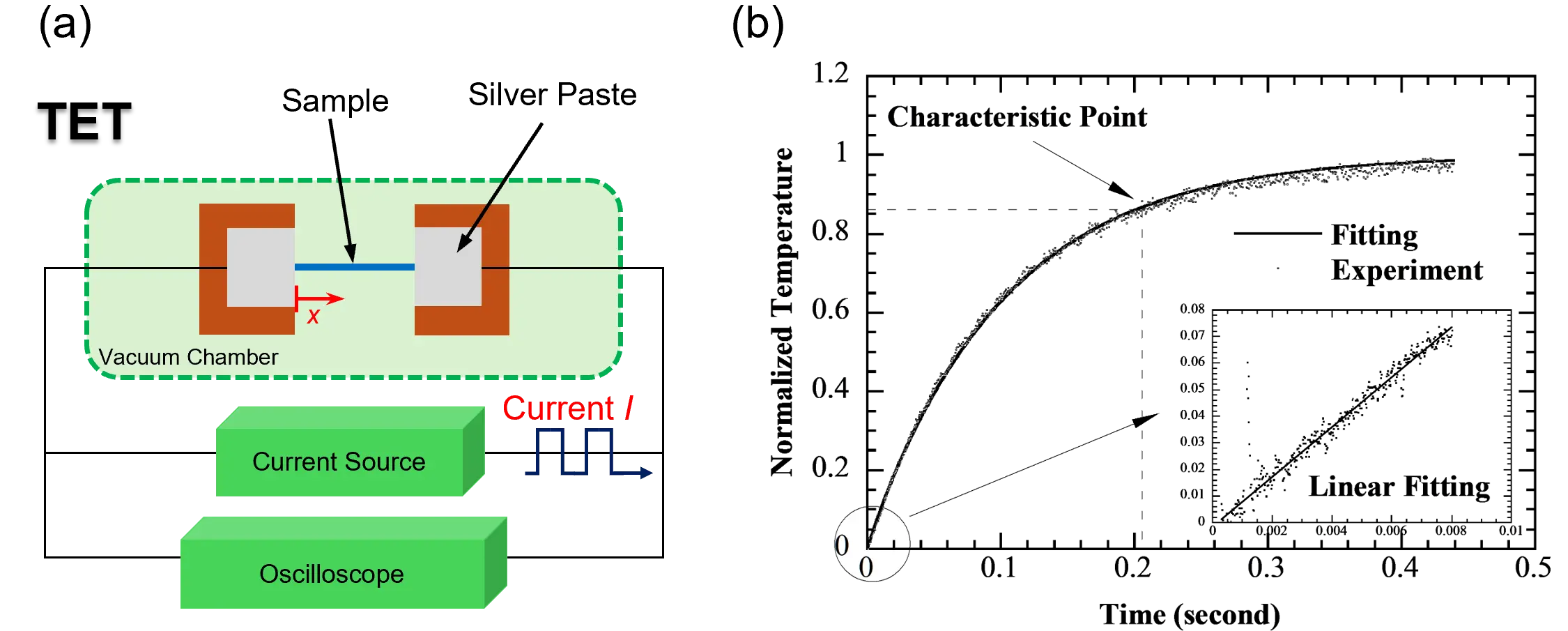
The second method is the characteristic point method. As shown by Eq. (6), the normalized temperature rise T^* depends solely on the term α_eff · t/L². This implies that a single, well-chosen point on the T(t) curve can be used to directly determine α_eff. The optimal characteristic point is where both T^* and t show maximum sensitivity to changes in α_eff. It has been demonstrated that this maximum sensitivity occurs when T^* = 0.8665, corresponding to a Fourier number of 0.2026^[14]. In this method, once the characteristic time t_c (the time at which T^*= 0.8665) is identified from the experimental data, α_eff can be calculated directly using α_eff = 0.2026L²/t_c. This method generally achieves higher accuracy by focusing on the point of greatest sensitivity on the normalized temperature curve, yielding an α_eff value close to the reference. It is also relatively robust against random data fluctuations, particularly when a small set of points surrounding the characteristic point is used to determine its position. However, the main drawback lies in the difficulty of precisely locating the characteristic point. Experimental noise often introduces uncertainties in determining t_c, which consequently affects the accuracy of the extracted α_eff.

The third method, the least squares fitting approach, provides the highest overall accuracy by globally fitting the entire V-t curve. By minimizing the total fitting deviation across the complete dataset, it achieves strong agreement with experimental results. However, this method is more complex and involves several steps, including identifying the heating start point (V₀), determining the steady-state voltage (V₁), and normalizing the experimental data. Each step can introduce additional errors and uncertainties, particularly if the steady-state voltage is not well defined or if the data are affected by noise. Consequently, although this method produces highly accurate α_eff values, it requires careful experimental control and meticulous data processing. To validate the TET technique and the associated data analysis methods, measurements were conducted on microscale Pt wires of varying lengths, with experimental conditions summarized in Table 2^[14]. All three data analysis methods described were applied to evaluate the α_eff of the Pt wire. Using the least squares fitting approach (method 3), the α_eff values for the three Pt wires were determined to be 2.53 × 10^-5, 2.54 × 10^-5, and 2.78 × 10^-5 m²/s, respectively^[14]. These results are in good agreement with the known literature value of 2.51 × 10^-5 m²/s at 300 K. Similarly, the characteristic point method (method 2) yielded comparable α_eff values of 2.47 × 10^-5, 2.41 × 10^-5, and 2.67 × 10^-5 m²/s for the same three samples.

Considering the limitations of the previously discussed data processing approaches, an alternative fitting method based on an exponential function has been developed. A simplified expression for the normalized average temperature rise of the sample, derived from Eq. (6), is given as:

(7)$T^{\ast }=1-\exp (-{\pi }^2{\alpha }_{eff}t/L^2)$

Since the transient voltage change of the sample is directly related to its temperature rise, the experimentally measured V-t data can be fitted using the following expression^[27]:

(8)$V=b_1+b_2\exp (-{\pi }^2{\alpha }_{eff}t/L^2)$

where b₁, b₂, and α_eff are the fitting parameters extracted during the curve-fitting process. It has been demonstrated that applying Eq. (8) to TET data fitting achieves high accuracy, with deviations less than 1%. Unlike the previous data processing methods, this approach eliminates multiple preprocessing steps, such as identifying V₀ and V₁ and normalizing the experimental data. Instead, all required parameters are obtained directly from the fitting procedure.

In TET measurements, the entire sample is uniformly heated, and the average temperature rise is used to determine α. This raises an important question: could variations in electrical resistance along the sample, which may occur naturally due to fabrication imperfections or material inconsistencies, influence the measured result? To address this, the Transient Photo-Electro-Thermal (TPET) technique was employed in our previous study to further examine the thermal diffusivity (α) of graphene fiber (GF)^[28]. Unlike the TET method, which uses step current-induced Joule heating, TPET employs step laser irradiation as the thermal excitation source. If the laser beam illuminates the entire sample, Eq. (6) remains applicable for calculating T^*. However, when the laser beam is confined to a width l, the solution for T^* is expressed as:

(9)$T^{\ast }=\frac{1}{Z}\sum _{m=1}^{\infty }\{\frac{\cos \left[\right(2m-1\left)\pi \xi /L\right]-\cos \left[\right(2m-1\left)\pi \right(\xi +l\left)/L\right]}{(2m-1{)}^4}\times [1-\exp (-(2m-1{)}^2{\pi }^2\alpha t/L^2)]\}$

Where

(10)$Z=\sum _{m=1}^{\infty }\left\{\frac{\cos \left[\right(2m-1\left)\pi \xi /L\right]-\cos \left[\right(2m-1\left)\pi \right(\xi +l\left)/L\right]}{(2m-1{)}^4}\right\}$

Here, ξ represents the position along the sample where the line-shaped laser beam is focused. In this implementation, a 532 nm laser (DPSS Inc.) was shaped into a narrow 0.1 mm-wide line using a cylindrical lens and focused on the sample to achieve localized heating. By systematically varying the laser incidence position along the fiber, we investigated its influence on the measured α_eff. The results, shown in Figure 2a, indicate that the measured thermal diffusivity remains nearly constant across all heating positions, except near the sample ends. This finding is significant because it confirms that for TPET-based thermal characterization of micro- and nanoscale wires, the position of laser heating does not substantially affect the outcome. Furthermore, this result addresses a potential concern regarding the TET method. Our TPET data clearly demonstrate that even when localized heating is applied at different positions, the extracted α remains consistent. Therefore, we conclude that local variations in electrical resistance along the sample do not meaningfully affect the thermal diffusivity results obtained using the TET method, further confirming its robustness.

Display Full Size

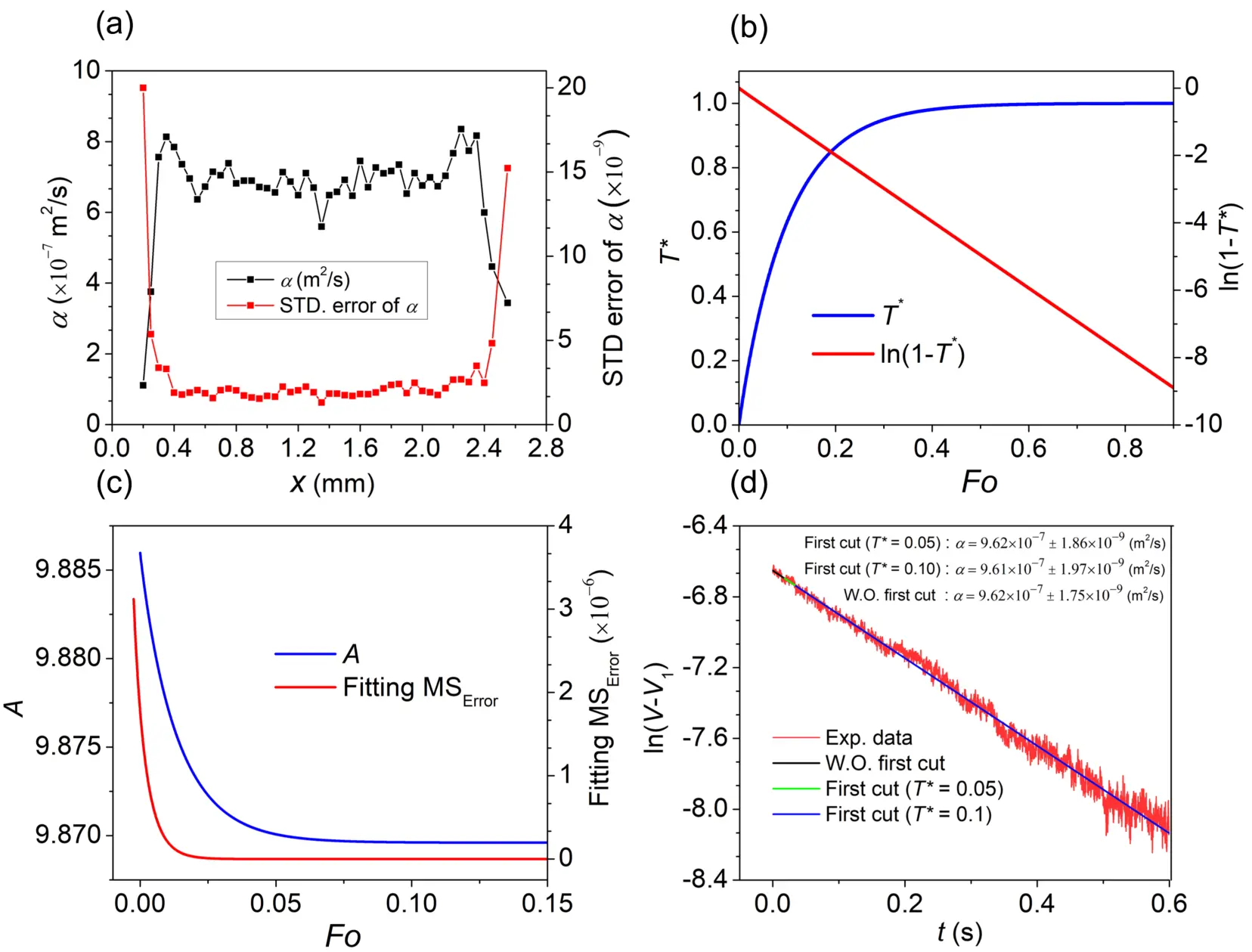
Figure 2. (a) Thermal diffusivities measured at different laser heating positions using the TPET method, with associated standard errors shown; (b) The linear-fitting-based approach introduced for TET signals data processing. The left axis shows the dimensionless temperature evolution plotted against Fo for the theoretical analysis of the TET method, while the right axis presents ln(1-T^*) vs. Fo from the same study; (c) The graph shows how the slope (coefficient A) from the linear fitting varies with Fo (left axis) and the corresponding MS_Error of the fitting (right axis); (d) Experimental data displaying the natural of GF TET voltage drop subtracted by the steady-state voltage plotted against time. Three different curve fitting strategies are shown: I) without removing the initial data, II) starting after T^* = 0.05, and III) starting after T^* = 0.1. The resulting thermal diffusivity values and their uncertainties are also included^[28]. TPET: Transient Photo-Electro-Thermal; TET: Transient Electro-Thermal; GF: graphene fiber.

There is an inherent uncertainty associated with the data-fitting process. For TET measurements, although α is obtained through nonlinear fitting of experimental data, directly determining the fitting uncertainty remains challenging. This difficulty arises in part from the highly complex relationship between temperature rise (or decay) and time, which complicates conventional uncertainty analysis. In most nonlinear least-squares fitting processes, the uncertainty of fitted parameters is quantified using the covariance matrix (COVB). After completing the fitting procedure, the Jacobian matrix (J) is computed, with each element representing the partial derivative of the fitting model with respect to a parameter, evaluated at the best-fit values. The product of the Jacobian transpose (J^T) and the Jacobian itself J^TJ reflects the model’s sensitivity to variations in the parameters. Inverting this matrix, (J^TJ)^-1, provides a measure of how uncertainties in the experimental data propagate into uncertainties in the estimated parameters. To account for the overall noise level in the measurements, the mean squared error (MSE) is calculated from the residuals between experimental data and model predictions. The COVB is then obtained by scaling the inverted sensitivity matrix by the MSE, following the relation: COVB = MSE × (J^TJ)^-1. The diagonal elements of the COVB correspond to the variances of each fitted parameter, and their square roots provide the standard deviations (i.e., the fitting uncertainties) for those parameters. It is important to note that this approach captures only the uncertainties arising from the fitting process itself, as our goal here is to evaluate fitting uncertainty specifically for comparison with the linear fitting method. If uncertainty propagation from input parameters (e.g., sample length) is also considered, the total variance can be expressed as: ${\sigma }_{ftt}^2+\sum _i{[\left(\partial \alpha /\partial x_i\right)\cdot {\sigma }_{x_i}]}^2$, where ${\sigma }_{fit}^2$ is obtained directly from the COVB of the nonlinear regression, and x_i and ${\sigma }_{x_i}$ are the input parameters and their respective uncertainties. These calculations not only increase computational cost but may also reduce precision. Several factors can compromise the accuracy and validity of such uncertainty estimates, one of the most significant being nonlinear effects. In nonlinear regression, uncertainty estimation assumes a reliable local linearization around the best-fit point. If the model exhibits strong nonlinearity, this approximation fails, and the computed covariance matrix may substantially underestimate the true uncertainties^[29].

In the next section, we introduce a rigorous approach developed to address these limitations. This method enables the extraction of both the thermal diffusivity and its associated uncertainty for microfibers and microwires by leveraging linear regression techniques for accurate uncertainty evaluation.

2.2 Mathematical treatment of the non-linear V-t data

In this section, we present a new linear-fitting-based approach for processing TET signal data, which enables the determination of both the fitting uncertainty and the resulting uncertainty in thermal diffusivity^[28]. The development of this method begins with establishing a theoretical framework. Figure 2b shows the theoretical curve of T^* versus the Fo, calculated using Eq. (6) for a given L and α. The figure also includes a secondary axis plotting ln(1-T^*) against Fo, which reveals a strong linear correlation and demonstrates the linearity inherent in the transformed relationship. At this point, one might question how the constant -π² appears in the exponential term of Eq. (7). In our earlier study, we considered a case in which a constant A (instead of -π²) appeared in Eq. (7), such that T^* = 1 - exp(-Aαt/L²). Rearranging this expression yields: ln(1-T^*) = -Aαt/L². This can also be expressed as: ln(1-T^*) = -A·Fo. Figure 2c illustrates that the value of A (which represents the slope) depends on the starting point of the fitting interval. Initially, A varies, but it eventually converges to a constant value of π². The graph on the right side of Figure 2c shows that, after Fo = 0.009 (corresponding to T^* = 0.1), the MS_Error of the linear fit becomes minimal and stabilizes. This observation supports the exclusion of data points corresponding to T^* < 0.1 when performing the linear regression.

Furthermore, the relationship between the TET voltage signal and T^* can be defined as: T^* = (V₀ - V)/(V₀ - V₁). Using this relationship, along with the theoretical behavior of ln(1-T^*) versus Fo, we developed a linear fitting method that provides an efficient and accurate approach for extracting α from TET measurements. This method involves applying a natural logarithmic transformation to the V-t signal and performing linear regression on the resulting curve, as defined by^[28]:

(11)$\ln |V-V_1|=-{\pi }^2{\alpha }_{eff}t/L^2+D$

This transformation effectively linearizes the TET signal. With the sample length L known, α_eff can be directly calculated from the slope of the fitted line, expressed as -π²α_eff/L². Compared to nonlinear global curve fitting, this approach not only simplifies the fitting procedure but also enables rigorous and accurate uncertainty estimation, which is otherwise challenging to achieve. The most accurate results occur when the data used for fitting fall within the normalized temperature rise range of 0.1 < T^* < 0.8, where the signal maintains strong linearity. Within this range, the typical fitting uncertainty is very small, often on the order of ± 0.5% or less. Figure 2d presents experimental data for ln(V-V₁) plotted against t from a TET test on a GF^[28]. Notably, once T^* = 0.8, the data begin to deviate from the expected linear trend, so these points are excluded from the fitting process. As indicated in Figure 2c, minor nonlinearity is also present at the beginning of the ln(1-T^*) ~ Fo relationship. To preserve the validity of assuming a constant π² in Eq. (11), early-stage data must also be excluded. To assess the effect of this exclusion on actual GF test data, linear fitting was performed under three different conditions: (1) using the full dataset, (2) excluding data with T^* < 0.05, and (3) excluding data with T^* < 0.1. The resulting α values were nearly identical, 9.62 × 10^-7, 9.62 × 10^-7, and 9.61 × 10^-7m²/s^[28], respectively (as shown in Figure 2d),confirming the robustness and reliability of this fitting method even when early-stage data are omitted.

In this work, to experimentally validate the accuracy and robustness of the proposed linear fitting method for extracting thermal diffusivity, a series of TET measurements were conducted on a well-characterized Pt wire sample. The Pt wire, purchased from Goodfellow Corp., has a diameter of D = 25.4 μm and a length of L = 10.192 mm, and was placed under vacuum conditions (< 0.2 mTorr). The electrical resistance of the sample was measured to be 2.70 Ω. TET measurements were performed at different current levels of 16, 18, 19, and 19.5 mA, with 10 repeated measurements at each current setting. These results will be discussed later in Section 6. In addition, the measurement at I = 18 mA was repeated 50 times, and the resulting signals were fitted using Eq. (11) to determine the α_eff of the sample. Because the emissivity of Pt wire at room temperature is very low (0.05-0.1), radiative heat loss is negligible; thus, the measured α_eff can be considered the intrinsic thermal diffusivity of the sample. Figure 3a presents representative examples of how ln(V-V₁) varies with t during TET experiments for the Pt wire at three current levels (16, 18, and 19 mA), along with the corresponding fitted curves. The extracted thermal diffusivity values and their standard errors (SE), obtained using Eq. (11), are 2.26 × 10^-5 ± 2.44 × 10^-8, 2.27 × 10^-5 ± 1.75 × 10^-8, and 2.20 × 10^-5 ± 1.53 × 10^-8 m²/s, respectively. It is important to note that the uncertainty (or SE) of the slope (-π²α_eff/L²) is calculated as: $\sqrt{S^2/\sum {(t_i-\overline{t})}^2}$, where $S^2=\sum {(Y_{fit}-Y_{act})}^2/(N-2)$. Here, N represents the total number of data points, Y_fit refers to the fitted values at each point, and Y_act denotes the $\ln |V-V_1|$ of the experimentally measured voltage values.

Display Full Size

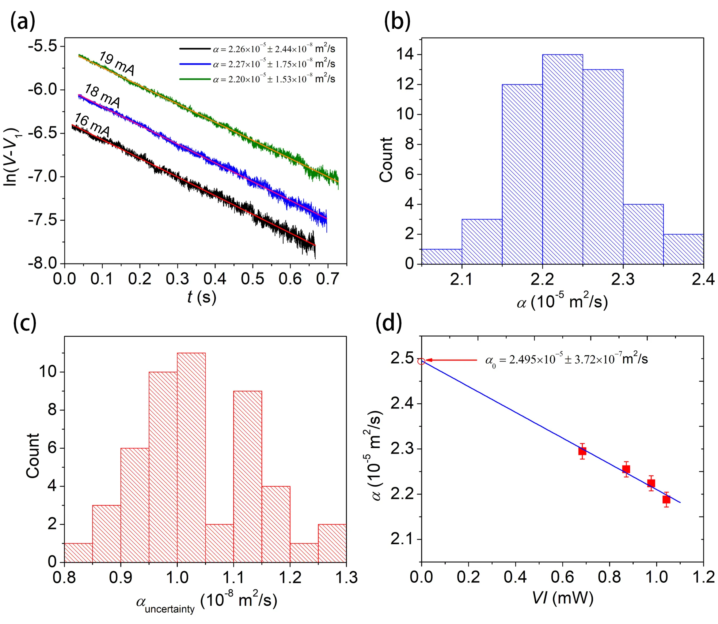
Figure 3. Experimental validation using a Pt wire confirming the robustness and reliability of the TET technique and the linear data processing approach. (a) Representative examples of ln(V-V₁) variation with t during the TET experiment for a Pt wire at three I values with their fittings. The resulting thermal diffusivities and uncertainties are also shown; The histogram shows the distribution of (b) the calculated α values and (c) the fitting uncertainties for the repeated Pt wire TET experiments; (d) The linear relationship between the average measured α and the corresponding heating power. The intercept of the α-VI linear fitting is used to extract the thermal diffusivity with zero temperature rise. TET: Transient Electro-Thermal.

The 50 repeated measurements on the Pt wire at a constant current of 18 mA were conducted to evaluate the consistency and reliability of the TET technique. Each V-t signal was analyzed by fitting the experimental data using Eq. (11) to extract the α and its associated fitting uncertainty. The results are summarized in the two histograms shown in Figure 3b and Figure 3c. Figure 3b illustrates the distribution of the calculated α values. The results yield an average α value (α_avg) of (2.30 ± 0.01) × 10^-5 m²/s, where the uncertainty represents the SE of the mean, computed as: $\mathrm{SE}=\mathrm{SD}/\sqrt{N}$, with SD defined as $\mathrm{SD}=\sqrt{\sum {({\alpha }_i-{\alpha }_{\text{avg}})}^2/(N-1)}$. The narrow distribution and low SE confirm that the fitting process is highly reproducible and that measurement noise is effectively suppressed. Figure 3c presents the histogram of the fitting uncertainties for the 50 trials. Most values fall between 0.9 × 10^-8 and 1.2 × 10^-8 m²/s, with a peak near 1.0 × 10^-8 m²/s, indicating a consistently high level of fitting precision across all measurements. Although the average thermal diffusivity of 2.30 × 10^-5 m²/s is lower than the literature value of 2.51 × 10^-5 m²/s at 300 K, this discrepancy does not represent an error. As will be discussed in Section 6, the measured α corresponds to conditions where the Pt wire experiences Joule heating during testing, which elevates the wire temperature and reduces its thermal diffusivity. Therefore, the reported average does not reflect the true value at ambient temperature. Section 6 introduces a method to extrapolate the results to zero temperature rise (Figure 3d), thereby recovering the true thermal diffusivity at ambient conditions and achieving better agreement with the reference value. Finally, both histograms exhibit no significant skewness or multimodal distribution, confirming that variations in α and fitting uncertainty primarily arise from random experimental and fitting noise rather than systematic errors.

Regarding the evaluation of contact resistance using silver paste, Guo et al.^[30] from our research group conducted a study to address this issue. In that work, they proposed a first-order approximation based on steady-state thermal resistance analysis. This simplified model estimates the effective thermal conductivity (k_eff) of the wire or microfiber under investigation as: $k_{eff}\approx k_w/(1+(D/L)\cdot \sqrt{k_w/\left(2k_b\right)})$. Here, k_w, D, and L represent the thermal conductivity, diameter, and length of the wire or microfiber, respectively. The term k_b denotes the thermal conductivity of the base, calculated as the average value of the thermal conductivities of the silver paste and the electrode material. The model indicates that the effective thermal conductivity depends on the wire’s aspect ratio (D/L) and the thermal conductivity ratio (k_w/k_b). When the base material has a much higher thermal conductivity (k_w/k_b << 1), the measured k_eff closely approximates the intrinsic value of the wire. This highlights the importance of selecting highly conductive electrode materials. Furthermore, the equation suggests that using thinner and longer wires (i.e., smaller D/L) further improves the accuracy of k_eff in representing the true thermal conductivity. Assuming the thermal conductivity of the Pt wire is approximately k_w ≈ 71.6 W/mK^[30], k_b ≈ 120.5 W/mK (with k_Al = 237 W/mK and k_{silver paste} = 4 W/mK), and and the wire dimensions are D = 25.4 µm and L = 10.2 mm, the estimated k_eff is 71.50 W/mK. This corresponds to a deviation of only about 0.14% from the intrinsic thermal conductivity of the Pt wire, indicating that the effect of thermal contact resistance in TET measurements is negligible.

In addition to fitting uncertainty, the total absolute uncertainty in thermal diffusivity measurements also accounts for errors in sample length (L) and variations in signal noise between repeated measurements. Among these factors, uncertainty in L is typically negligible, and the high repeatability of the TET system ensures that signal variations across multiple tests remain well controlled, generally within ±1%. This overall robustness makes the linear fitting approach both accurate and highly repeatable for quantitative TET-based thermal analysis.

2.3 Physics model of TET for measuring semiconductive materials

For many materials, the TET signal (V-t) exhibits purely monotonic behavior, either increasing or decreasing, depending on the temperature coefficient of resistivity (θ_T = dρ_e/dT), where ρ_e denotes electrical resistivity. When the temperature change during a TET measurement is small, θ_T can generally be assumed constant. However, for certain materials, particularly semiconductors, the transient response can deviate markedly from this ideal behavior, resulting in abnormal TET signal profiles. The underlying physical reason is that θ_T does not remain constant during the TET process; instead, it may vary significantly or even change sign. This occurs because θ_T depends on how both the carrier concentration (n) and the electron scattering time (τ) vary with temperature (T). The electrical resistivity ρ_e is expressed as ρ_e = m/(ne²τ), where m is the electron mass and e is the electron charge. As T increases, more electrons are excited into the conduction band, increasing n. Meanwhile, τ is affected by electron scattering, which arises from defects, impurities, and phonons (lattice vibrations). While defect and impurity scattering are largely temperature-independent, phonon scattering intensifies with increasing T because more phonons are generated. As a result, dτ/dT is expected to be negative. Consequently, the combined temperature effects on n and τ can cause θ_T to switch signs within a certain T range in semiconductive materials. This sign reversal in θ_T explains the abnormal TET signal behavior observed during measurements.

For conventional TET measurements where resistance R varies linearly with T, the change in electrical resistivity (Δρ_e) can be expressed as Δρ_e = θ_TΔT. This leads to a direct linear relationship between the change in resistance (ΔR) and the average temperature rise ($\overline{\Delta T}$) of the sample, given as $\Delta R={\theta }_T\beta \overline{\Delta T}$, where β = L/A and A is the cross-sectional area of the sample. Based on Eq. (7), the average temperature rise of the sample can be expressed as^[27]:

(12)$\overline{\Delta T}=a_1+a_2\exp (-{\pi }^{2}Fo)$

Here, a₁ and a₂ are fitting constants. Since changes in R and V during TET are linearly related to T, the transient ΔV can also be expressed in the same form as $\overline{\Delta T}$. To verify the validity of Eq. (12), a theoretical calculation was performed using Eq. (2) by simulating the temperature rise at 25 equally spaced points along a sample, with fixed values of q̇, α, and k. The results, shown in Figure 4a, illustrate the evolution of temperature rise at different positions along the sample. Figure 4b presents the nature of the difference between steady-state and transient temperature rise as a function of Fo at various selected locations. The slope of these plots is used to assist in formulating the analytical model. Note that ξ = x/L. Using these values, the $\overline{\Delta T}$ was computed and fitted perfectly using Eq. (12), as shown in Figure 5a, demonstrating the accuracy of this equation^[27].

Display Full Size

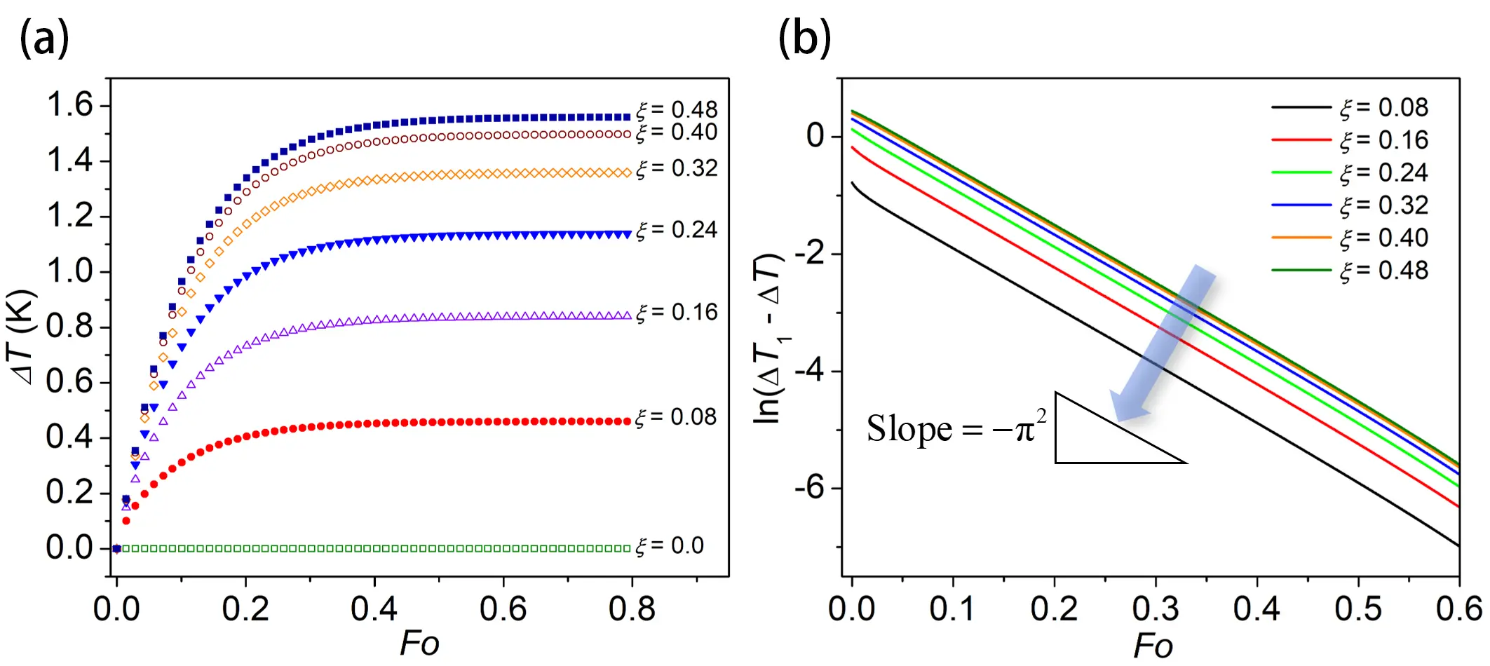
Figure 4. Demonstration of the validity of the physics model of TET in Eq. (12) for measuring semiconductive materials based on theoretical calculation. (a) Calculated temperature profiles at various normalized positions along the sample (ξ = x/L) based on the theoretical solution of the TET method; (b) Natural of the difference between the steady-state temperature rise and the transient temperature rise is plotted against Fo for several selected positions. The slope of these curves is used to support the development of the analytical model^[27]. TET: Transient Electro-Thermal.

Display Full Size

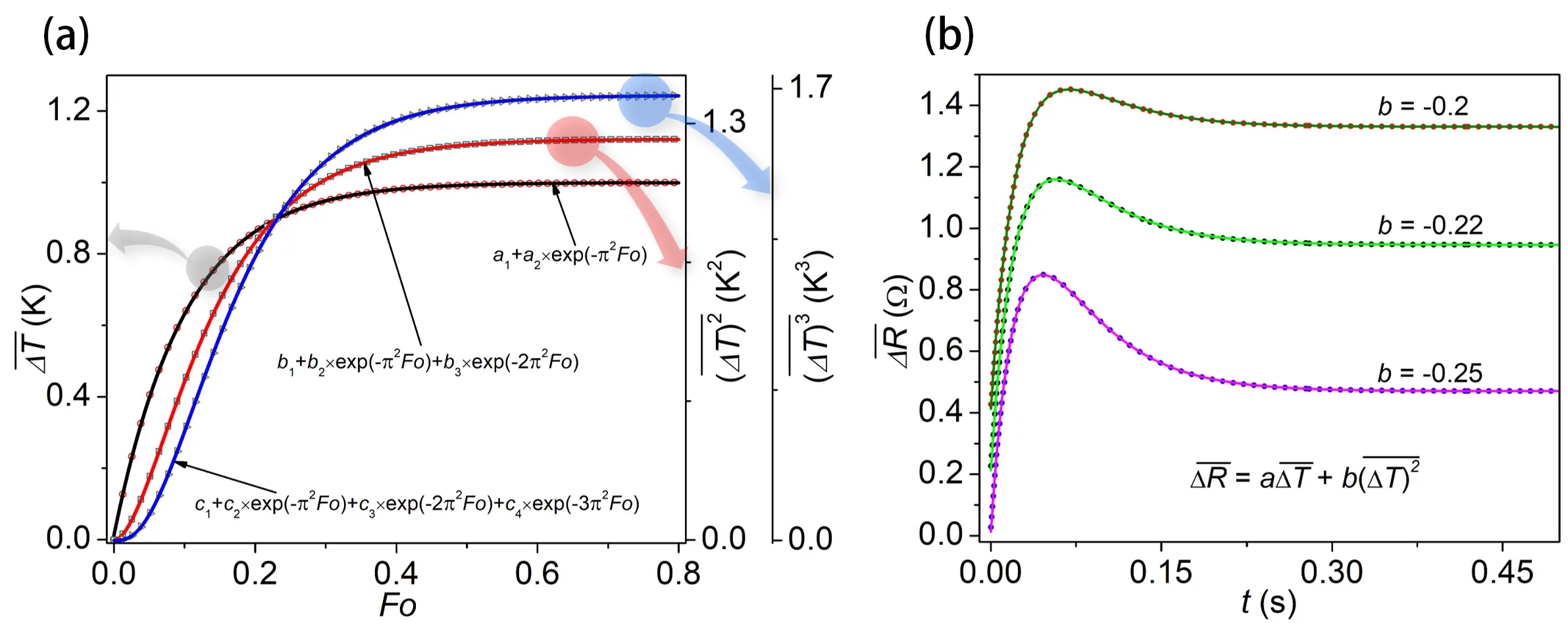
Figure 5. The validity of the developed TET theory under a higher order of dependency of ρ_e on T based on theoretical calculations. (a) Displays the mean temperature rise (left axis), the mean squared temperature rise (first right axis), and the mean cubed temperature rise (second right axis) of the sample, computed from the temperature profiles at various positions. The corresponding fitted curves for each case are shown as solid lines; (b) Shows the simulated average resistance change over time (dots) for a 1D sample, modeled numerically while applying different values of the parameter b. The fitted curves for these resistance-time (R-t) responses are shown as solid lines. To enhance clarity, offsets of +0.4 Ω and +0.2 Ω were added to the b = -0.2 and b = -0.22 cases, respectively^[27]. TET: Transient Electro-Thermal; 1D: one-dimensional.

When abnormal TET signals are observed, meaning ΔR does not exhibit a linear correlation with ΔT, a higher-order dependency of ρ_e on T is assumed: Δρ_e = ɑΔT + b(ΔT)². Integrating this over the sample length, the total resistance change becomes $\Delta R=\beta [a\overline{\Delta T}+b\overline{(\Delta T{)}^2}]$. Note that the average squared temperature rise, $\overline{(\Delta T{)}^2}$, must first be calculated by squaring the temperature rise at each point and then averaging it. Another expression was proposed to fit this profile as^[27]:

(13)$\overline{(\Delta T{)}^2}=b_1+b_2\exp (-{\pi }^2{F}_O)+b_3\exp (-2{\pi }^2{F}_O)$

The design of Eq. (13) directly follows from Eq. (12). Squaring the local temperature rise preserves the exponential terms but elevates them to higher orders, which naturally leads to the form of Eq. (13). Similar to Section 2.2, another theoretical analysis showed that the slope of ln(ΔT₁-ΔT) versus Fo at different sample locations remains consistently -π², as illustrated in Figure 4b. This provides additional evidence for the occurrence of -π² in the exponential terms. Here, ΔT₁ represents the steady-state temperature rise at each location. Consequently, ΔR can also be expressed as a combination of two exponential terms. For stronger nonlinearities, a third-order relationship can be assumed: Δρ_e = ɑΔT + b(ΔT)² + c(ΔT)³. For $\overline{(\Delta T{)}^3}$, this can be expressed as^[27]:

(14)$(\overline{\Delta T{)}^3}=c_1+c_2\exp (-{\pi }^2{F}_O)+c_3\exp (-2{\pi }^2{F}_O)+c_4\exp (-3{\pi }^2{F}_O)$

The theoretical calculations for $\overline{(\Delta T{)}^2}$ and $\overline{(\Delta T{)}^3}$, along with their corresponding fittings using Eq. (13) and Eq. (14), are presented in Figure 5a^[27].

Consequently, the total resistance change considering third-order terms follows the form^[27]:

(15)$\overline{\Delta R}=g_1+g_2\exp (-{\pi }^{2}Fo)+g_3\exp (-2{\pi }^{2}Fo)+g_4\exp (-3{\pi }^{2}Fo)$

Since V is linked to the change in R as $V=I_0\cdot \overline{\Delta R}+V_0$, the measured V~t data can be modeled as^[27]:

(16)$V=f_1+f_2\exp (-{\pi }^{2}Fo)+f_3\exp (-2{\pi }^{2}Fo)+f_4\exp (-3{\pi }^{2}Fo)$

Eq. (16) enables the fitting of experimental TET signals even under abnormal, nonlinear conditions. It is noteworthy that in most cases, a second-order nonlinearity is sufficient to capture the sample behavior, as this is more common and physically realistic within the small temperature changes typically encountered in practical TET measurements.

The validity of the developed theory was verified through a numerical TET simulation^[27]. A numerical program was used to compute the R-t response of a sample under nonlinear R-T behavior. The model was capable of incorporating spatial variations of properties such as k, ρc_p, and θ_T along the sample’s length. However, for simplicity, all properties were assumed constant except for θ_T. The simulation employed the finite volume method with an implicit algorithm. The R-T relationship was modeled as nonlinear, following Δρ_e = aΔT + b(ΔT)², where a = 1 and b was varied as -0.2, -0.22, and -0.25. The simulated R-t responses for different b values were plotted as dots in Figure 5b. These profiles were then fitted using Eq. (15), considering only the first two exponential terms. The fitting results, shown as solid lines in Figure 5b, matched the simulated data very well. For the simulation, the actual α of the sample was 2 mm²/s. Remarkably, the values of α obtained from the fitting procedure closely matched the modeled α, with deviations of less than 0.5%. This high level of agreement strongly confirms the validity of the developed physical model for analyzing abnormal TET signals.

Subsequently, the theoretical model developed earlier was successfully applied to fit the experimental TET signals (V-t) of the graphene film (GreF) sample^[27]. The GreF sample was electronically conductive, eliminating the need for a metallic coating. At low temperatures (e.g., 84.5 K), the TET signal for GreF exhibited a smooth, monotonically decreasing trend, which could be effectively modeled using the single exponential term in the proposed expression [Eq. (8)]. This occurred before reaching a transition range where the TET signal began to exhibit abnormal behavior (Figure 6a, Figure 6b and Figure 6c). The extracted α values showed a clear decreasing trend with increasing temperature from 84.5 K to 503 K, as shown in Figure 6d. However, beyond approximately 530 K, the TET signals displayed an abnormal and complex profile due to a semiconductive-to-metallic transition. Within this transition zone (approximately 530-630 K), the voltage behavior shifted from a purely decreasing trend to an abnormal form, and then to an increasing trend above about 630 K, reflecting a sign change in θ_T (from negative to positive). This behavior indicated changes in the dominant carrier transport mechanisms, as further confirmed by the R-T relationship shown in Figure 6e. To address the abnormal signal behavior in this regime, Eq. (16) with the first two exponential terms was employed. The resulting two-exponential function provided excellent fits for experimental signals at 560.6 K, 584.4 K, and 602 K (see Figure 6a, Figure 6b and Figure 6c). The corresponding α values obtained from these fittings (red squares in Figure 6d) formed a smooth and continuous trend across the transition, validating the robustness of the model in capturing abnormal TET behaviors. Furthermore, the α-T behavior was interpreted using the thermal reffusivity (Θ = 1/α) framework, providing insights into the phonon transport mechanisms in carbon-based materials such as GreF. Collectively, these results confirm that the two-exponential V-t model, grounded in the physical theory of carrier transport and phonon scattering, can reliably capture abnormal TET responses in semiconductive materials^[27].

Display Full Size

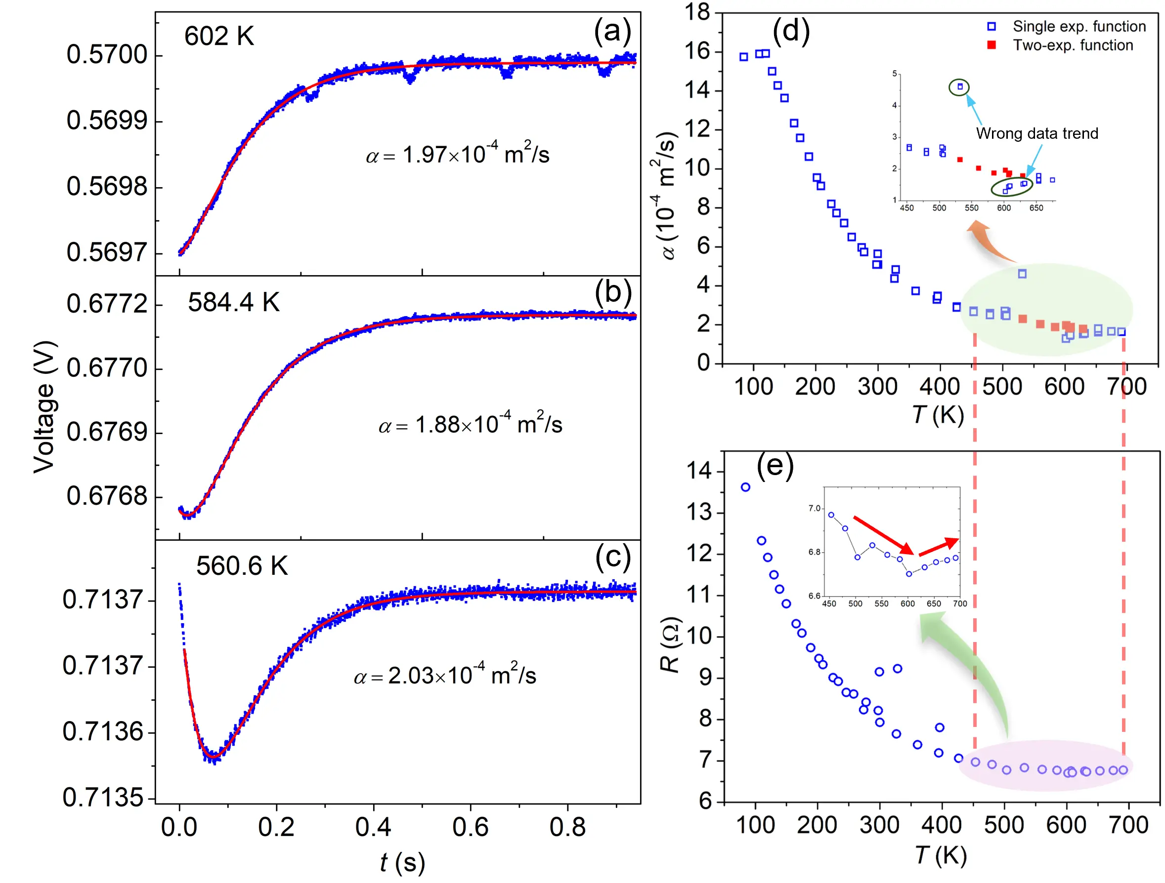
Figure 6. Demonstration of the two-exponential V-t model developed for fitting the experimental TET signals (V-t) of the GreF sample with a reversed sign of θ_T. (a-c) Present the TET signal responses of a GreF sample at three different temperatures: 602 K, 584.4 K, and 560.6 K, along with the fitting curves obtained using a two-exponential function; (d) Shows how the thermal diffusivity of the GreF sample varies with temperature, calculated using both single- and two-exponential fitting methods. The inset highlights the inaccuracy of the single-exponential approach for determining thermal diffusivity; (e) Displays the resistance change of the GreF sample as a function of temperature, with the inset revealing a sign reversal in the temperature coefficient of resistance (θ_T) near 600 K^[27]. TET: Transient Electro-Thermal; GreF: graphene film.

3. Stray Heat Transfer Consideration

3.1 Effect of radiation and convection heat transfer

During TET characterization, thermal radiation and air convection heat transfer can also influence the temperature evolution. Under typical experimental conditions, where the test chamber maintains a high vacuum (< 0.1 Pa), convective heat transfer through air becomes negligible. The thermal radiation term is also negligible at low temperatures, as it is substantially suppressed compared to the Joule heating power. However, at higher temperatures, thermal radiation becomes significant for samples with high aspect ratios or low thermal conductivity, where radiation markedly affects the temperature distribution and measurement accuracy. Both radiative and convective heat transfer can be calculated and subsequently excluded from the measured thermal diffusivity or conductivity results. By converting surface radiation and air convection into volumetric cooling sources, the heat transfer governing equation can be expressed as^[14,31]:

(17)$\frac{1}{\alpha }\frac{\partial \theta (x,t)}{\partial t}=\frac{{\partial }^2\theta (x,t)}{\partial x^2}+\frac{I^2{R}_0}{kL{A}_c}+\frac{Q_{\mathrm{rad}}}{k{A}_c}+\frac{Q_{\mathrm{cov}}}{k{A}_c}$

Here, R₀ is the resistance of the sample before Joule heating, and A_c is the cross-sectional area of the sample. Q_rad and Q_cov represent the heat transfer rates by radiation and air convection, respectively. The radiative heat transfer Q_rad can be deduced as:

(18)$Q_{\text{rad}}={\epsilon }_r\sigma A_s(T^4-T_0^4)={\epsilon }_r\sigma A_s(4T_0^3\theta +6T_0^2{\theta }^2+4T_0{\theta }^3+{\theta }^4)$

Here, ε_r the effective emissivity of the sample’s surface, σ = 5.67 × 10^-8 W/m² K⁴ is the Stefan-Boltzmann constant, and A_s is the surface area. In most cases during TET characterization, the temperature rise θ is much smaller than the ambient temperature T₀. Therefore, Q_rad can be further simplified as $Q_{\text{rad}}\approx 4{\epsilon }_r\sigma A_s{T}_0^3\theta$. In addition, if the air pressure in the vacuum chamber is not sufficiently low, thermal convection by air will also influence the temperature evolution during TET characterization. Under this condition, Q_cov can be calculated as: Q_cov = hA_sθ, where h is the thermal convection coefficient.

Substituting $Q_{\text{rad}}\approx 4{\epsilon }_r\sigma A_s{T}_0^3\theta$ and Q_cov = hA_sθ into Eq. (17), and solving the partial differential equation by integration of Green’s function, the effective thermal diffusivity α_eff is obtained as α_eff = α(1 - f), where f is defined as $f=-(4{\epsilon }_r\sigma T_0^3+h)A_{s}L/\left({\pi }^2{A}_{c}k\right)$. Therefore, α_eff can be expressed as a combination of the real thermal diffusivity α_real, the thermal radiation effect, and the thermal convection effect:

(19)${\alpha }_{eff}={\alpha }_{\text{real}}+\frac{4{\epsilon }_r\sigma T_0^{3}L}{{\pi }^2\rho c_p}\frac{A_s}{A_c}+\frac{hL}{{\pi }^2\rho c_p}\frac{A_s}{A_c}$

The second term on the right-hand side represents the thermal radiation effect, while the third term accounts for the thermal convection effect. For samples with rectangular cross-sections (such as films with width W, thickness δ, and suspended length L), the surface area can be approximated as A_s ≈ 2WL, and the cross-sectional area as Ac = Wδ. Therefore, for films-like samples, Eq. (19) becomes:

(20)${\alpha }_{eff}={\alpha }_{\text{real}}+\frac{8{\epsilon }_r\sigma T_0^3{L}^2}{{\pi }^2\rho c_p\delta }+\frac{2h{L}^2}{{\pi }^2\rho c_p\delta }$

For samples with round cross-sections (such as fibers or bundles with diameter D and suspended length of L), we have A_s = πDL and A_s = πD²/4. Thus, for round cross-section samples, Eq. (19) becomes:

(21)${\alpha }_{eff}={\alpha }_{\text{real}}+\frac{16{\epsilon }_r\sigma T_0^3{L}^2}{{\pi }^2\rho c_{p}D}+\frac{4h{L}^2}{{\pi }^2\rho c_{p}D}$

Eq. (20) and Eq. (21) demonstrate that the effective thermal diffusivity α_eff has a linear relationship with both radiation and air convection effects. Furthermore, these effects are proportional to L²/δ for films and L²/D for fibers or bundles. Thus, the contributions of radiation and convection can be determined and subtracted from α_eff using a differential method, by measuring the same sample with different suspended lengths.

The differential method of the TET technique has been employed to measure the thermal radiation effect in porous carbon materials^[31-34] and very thin fibers or films^[35], where thermal radiation significantly influences heat transfer. Lin et al.^[31] first proposed this differential method in 2013 to subtract the thermal radiation effect and obtain the intrinsic thermal diffusivity of the skeleton of porous graphene foams. By measuring graphene foam samples with different suspended lengths under vacuum conditions (where air convection is negligible), the radiation effect was determined and excluded from α_eff. Later, Liu et al.^[35] characterized the thermal conductivity k of giant chemical vapor deposition (CVD) synthesized graphene supported on poly(methyl methacrylate) (PMMA) using the TET technique in vacuum. The thermal radiation effect and surface emissivity were evaluated based on the differential concept. As shown in Figure 7, graphene samples measured at different suspended lengths using the TET technique exhibited a strong linear relationship between α_eff and the square of the suspended length (L²). According to Eq. (20), the intercept on the α_eff-L² plot corresponds to the intrinsic thermal diffusivity α_real of the sample. Moreover, the slope of the α_eff-L² curves was used to determine the emissivity of the four graphene samples. Therefore, the differential method in the TET technique not only effectively eliminates interference from thermal radiation but also enables simultaneous measurement of the material’s surface emissivity. It is worth noting that terms such as “1.33-layered” or “1.53-layered” refer to the average number of graphene layers across a sample with some degree of layer non-uniformity. These values do not represent discrete, physically fractional atomic layers; rather, they reflect statistical averages calculated from a population of regions within the sample. As described, Raman spectroscopy was performed at multiple random locations on each sample to estimate the number of graphene layers based on the intensity ratio of the G and 2D peaks (I_G/I_2D)^[35]. For instance, in one sample, 53.3% of the area consisted of single-layer graphene, 40.0% of double layers, and 6.7% of triple layers, resulting in a weighted average of 1.53 layers.

Display Full Size

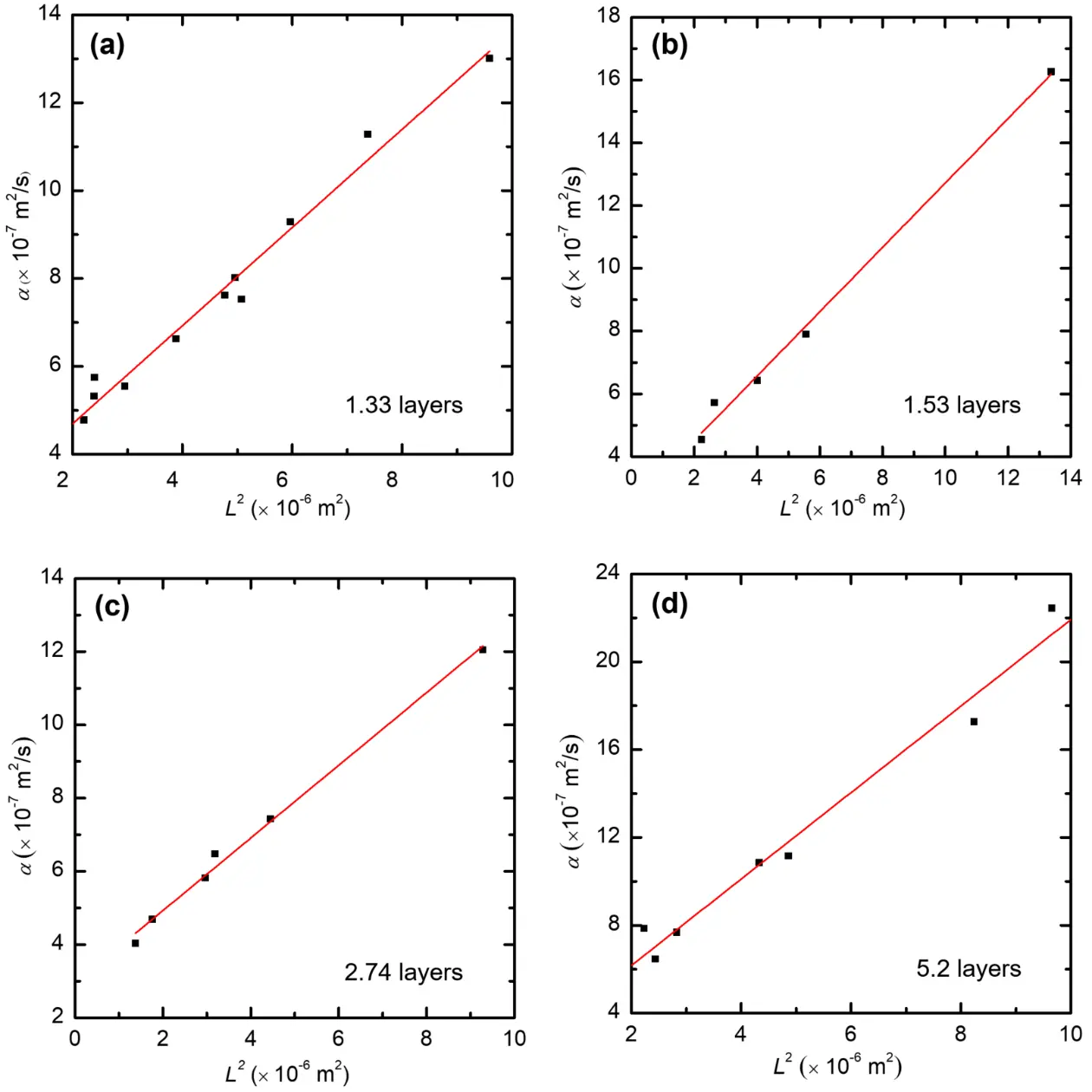
Figure 7. One representative example of ruling out the radiation effect and determining the surface emissivity simultaneously. Graphene samples supported on a PMMA film were measured at different suspended lengths, where α_eff-L² presented a good linear relationship, including (a) 1.33-layered graphene; (b) 1.53-layered graphene; (c) 2.74-layered graphene; (d) 5.2-layered graphene. Black dots are the experimental data, and red lines are the linear fitting^[35]. PMMA: poly(methyl methacrylate).

It should be noted that the significance of the thermal radiation effect depends on both the value of α_real and the aspect ratio of the sample under test. A larger L²/δ (for films) or L²/D (for fibers or bundles) results in a more pronounced thermal radiation effect. Furthermore, for materials with extremely low α_real (i.e., very low thermal diffusivity or conductivity), thermal radiation becomes non-negligible compared to thermal conduction during TET characterization, and it may even exceed 100% of the heat transfer contributed by conduction, necessitating special consideration. To accurately quantify the radiation effect, measurements should be performed on samples with at least three different suspended lengths to allow linear fitting of the α_eff-L² relationship. Using the same approach, the effect of air convection can also be quantitatively evaluated by systematically varying the suspended length, enabling simultaneous determination of the convection heat transfer coefficient.

3.2 Effect of electrically conductive coating

The TET technique can also be applied to non-conductive materials. Prior to measurement, a nanometer-thick metallic film (e.g., gold or iridium) is deposited on the surface of the sample to enable Joule heating and temperature evolution sensing. The influence of this metallic coating must be quantified and subtracted from α_eff. In practice, the measured α_eff represents the combined effect of the sample and the metallic thin film, which can be expressed as^[14]:

(22)${\alpha }_{eff}=\frac{k(1-\chi )+k_f\chi }{\rho c_p(1-\chi )+{\rho }_f{c}_{p,f}\chi }$

Here the subscript “f” is for the metallic film. χ is the cross-sectional area ratio of the metallic film, which can be calculated as χ = A_f/(A_f + A_c), where A_f is the cross-sectional area of the metallic film, and A_c is the cross-sectional area of the sample without coating. Since the metallic film is only a few nanometers thick (χ << 1), this relationship can be simplified as:

(23)${\alpha }_{eff}\approx \frac{k+k_f\chi }{\rho c_p}=\alpha +\frac{k_f\chi }{\rho c_p}$

Here α is the real thermal diffusivity of the sample, and the second term accounts for the metallic coating effect. The thermal conductivity of the metallic film (k_f) can be determined using the Wiedemann-Franz law: L_Lorenz = k_f/σT, where L_Lorenz is the Lorenz number of metal. σ is the film’s electrical conductivity, and can be readily determined as σ = L/(A_fR). Therefore, α_eff can be expressed as:

(24)${\alpha }_{eff}=\alpha +\frac{L_{\text{Lorenc}}TL}{R{A}_c\rho c_p}$

Here, T and R represent the average temperature and resistance during TET characterization. Based on Eq. (24), the contribution of the metallic coating can be accurately calculated and eliminated.

Furthermore, based on the above equation, it is evident that α_eff is linearly related to the inverse of resistance (R^-1). Thus, the influence of the metallic coating can also be eliminated using a differential TET method by varying the coating thickness. By linearly fitting the α_eff-R^-1 data points and extrapolating to R^-1 = 0 (corresponding to zero coating thickness), the intrinsic thermal diffusivity of the sample can be obtained at the intercept. Additionally, the slope of the α_eff-R^-1 relationship depends on the Lorenz number of the metallic film, providing a reliable approach for characterizing the Lorenz number of nanometer-scale metallic films^[36,37]. Lin et al.^[36] employed this method in 2013 to simultaneously determine the thermal and electrical conductivities, as well as the Lorenz number, of polycrystalline iridium (Ir) films with average thicknesses ranging from 0.6 to 7 nm. By successively depositing Ir layers on the same glass fiber and measuring the corresponding thermal diffusivity, five α_eff values were obtained. As shown in Figure 8a, α_eff exhibited a strong linear correlation with R^-1. Figure 8b and Figure 8c present the linear fitting curves of α_eff and R^-1 as a function of the number of Ir layers applied to the glass fiber. Based on these measurements, the thermal and electrical conductivities of Ir films were characterized down to an average thickness of 0.6 nm, revealing reductions of 82% and 50%, respectively, compared with bulk values. The Lorenz number of the 0.6 nm Ir film was measured to be 7.08 × 10^-8 WΩ/K², nearly twice the bulk value.

Display Full Size

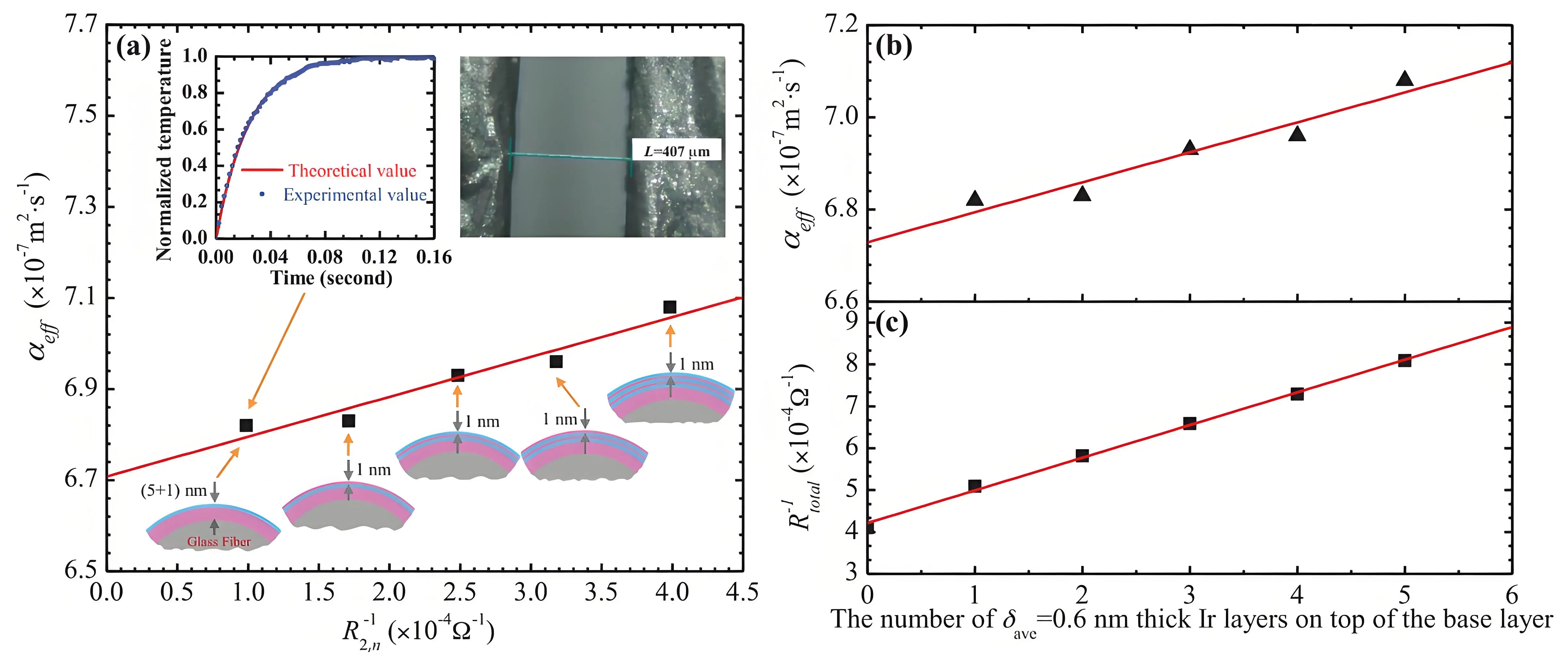
Figure 8. One representative example of ruling out the effect of metallic coatings and determining the Lorenz number of nm-thick metallic films based on a differential TET method by varying the number of 0.6-nm Ir coating layers. (a) α_eff against R^-1 of Ir-coated glass fiber by varying the Ir coating thickness; (b), (c) α_eff and R^-1 against the number of 0.6 nm Ir coatings on top of the base glass fiber, respectively. The suspended Ir-coated glass fiber under optical microscope is shown in the upper right inset in (a). The fitting of the normalized temperature rise (one layer of 0.6-nm Ir coating) is presented in the upper left inset in (a)^[36]. Dots: experimental data, red lines: linear fitting. TET: Transient Electro-Thermal.

4. Down to Atomic-thick Material Measurement: Differential TET

In TET measurements, the sample must be suspended between two electrodes to satisfy the physical model requirements. However, when the sample becomes extremely thin, on the order of a few nanometers or less, such a configuration becomes impractical or extremely challenging. In these cases, a differential TET methodology can be employed: the target sample is supported by another material to enable the construction of a bridge configuration. After the effective thermal diffusivity (α_eff) is measured, the sample’s thermal conductivity can be calculated using Eq. (22) by subtracting the contribution of the supporting material. To maximize the accuracy of this measurement, the supporting material should be as thin as possible and exhibit minimal thermal conductivity. This strategy was adopted by Liu et al.^[35] for measuring the thermal conductivity of mono- to few-layer graphene. In their study, the graphene sample was supported on an ultra-thin PMMA film (approximately 600-800 nm thick) with a thermal conductivity of about 0.21 W/mK. This configuration allowed the thermal conductivity of graphene to be measured with high confidence down to 33.5 W/mK. The effect of the supporting layer can be estimated as follows: assuming a PMMA thickness of 700 nm and a graphene thickness of 1.5 nm with a thermal conductivity of 33.5 W/mK, the effective in-plane thermal conductivity of the composite is approximately 0.281 W/mK, which is about 34% higher than that of the supporting material alone. Such a difference is easily detectable using the TET technique, which offers an accuracy of 1% or better. Based on this analysis, it is evident that the differential TET approach can be applied to measure the thermal conductivity of most two-dimensional materials with an accuracy far superior to that of Raman scattering-based methods. It should be noted that convection effects were negligible because the experiment was conducted under high vacuum (< 0.5 mTorr). In addition, the influence of thermal radiation was eliminated by measuring samples of different lengths.

Figure 9 illustrates the variation in thermal conductivity of supported graphene measured using the differential TET technique, its dependence on material thickness, and its corresponding electrical conductivity^[35]. This dataset represents some of the most accurate measurements of supported graphene to date. Moreover, it revealed a surprising linear correlation between thermal and electrical conductivities. Our subsequent studies confirmed that this linear relationship holds true for various carbon-based materials, including carbon nanotubes (CNTs), carbon fibers, and carbon nanocoils. This behavior is attributed to the significantly suppressed thermal and electrical conductivities in amorphous regions and along the c-axis of the crystalline structure^[38,39]. Additionally, the differential TET method has been successfully applied to measure the thermal conductivity of ultra-thin metallic coatings with thicknesses of just a few nanometers^[36,40-44]. These studies revealed non-uniform boundary scattering of electrons at grain boundaries affecting both heat and charge transport, a substantial increase in the Lorenz number of nanostructured films, and electron hopping mediated by organic substrates.

Display Full Size

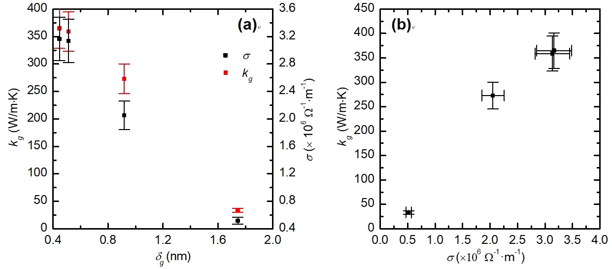
Figure 9. The thermal conductivity of graphene measured using the differential TET technique. The graphene samples were supported on an extra-thin PMMA film (~600-800 nm) to make it possible to construct the bridge configuration. The sample has a rectangular geometry, ~1 mm in width and ~2 mm in length. (a) The variation of thermal conductivity and electrical conductivity against graphene thickness. (b) The variation of thermal conductivity against its electrical conductivity^[35]. PMMA: poly(methyl methacrylate); TET: Transient Electro-Thermal.

5. Dynamic Heat Conduction within the Material

With its exceptional temporal resolution (typically < 1 s per measurement), the TET technique provides a powerful tool for real-time characterization of dynamic heat conduction behavior in materials. Material processing methods such as thermal annealing, laser treatment, and chemical, electrical, or magnetic modifications often involve complex microstructural evolution, including thermal stress, grain growth, phase transitions, defect aggregation, and changes in orientation, which are challenging to capture dynamically. Consequently, the development of advanced in-situ thermal characterization techniques capable of monitoring real-time microstructural changes and dynamic variations in thermal conductivity during processing is essential for achieving precise control.

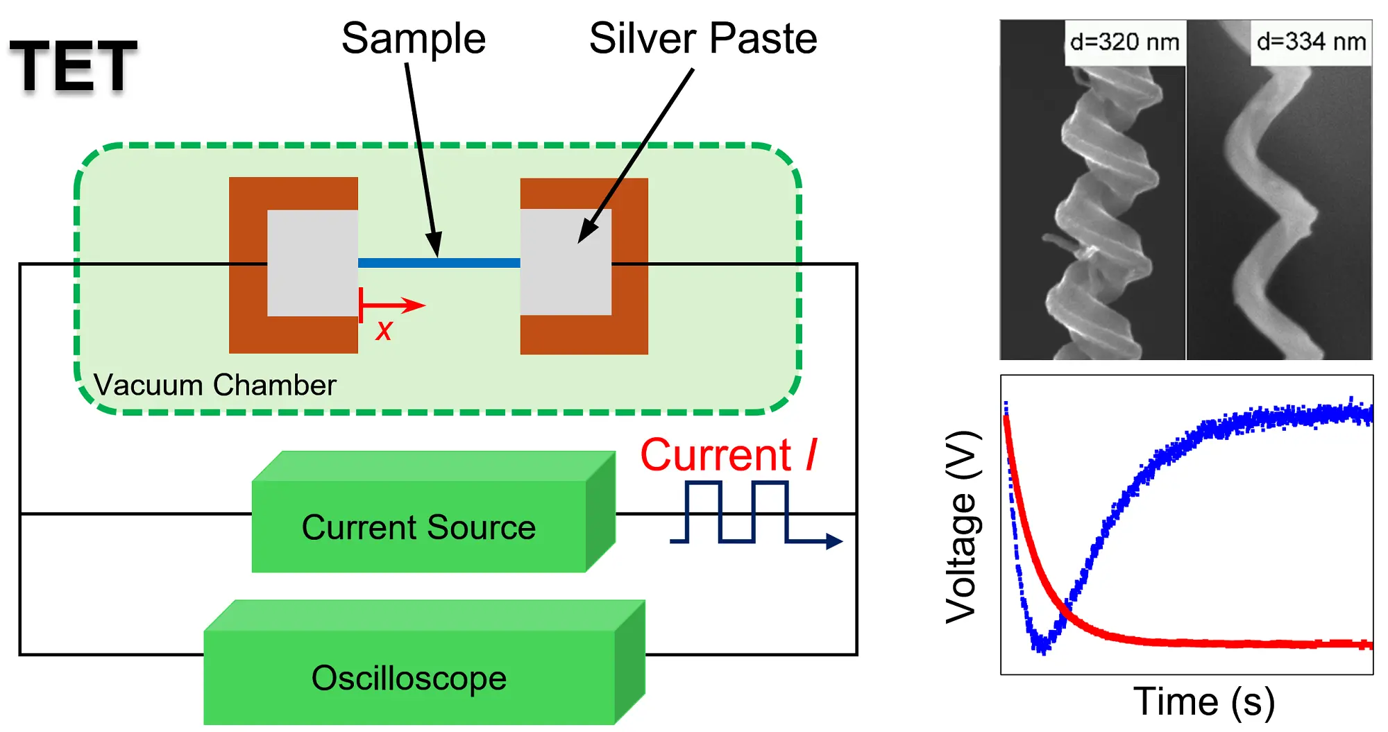
The dynamic thermal and electrical evolution of CNT bundles^[25] and carbon fibers^[45] during Joule heating-induced thermal annealing, as well as graphene aerogel (GA) microfibers during laser photoreduction^[18], have been investigated using in-situ TET characterization in recent years. Processes involving chemical structural changes can also be monitored dynamically. For example, biomass pyrolysis is a heat-intensive chemical reaction process in which the heating rate significantly influences the yield and composition (or quality) of the resulting biofuel. Xu et al.^[46] developed a continuous in-situ thermal characterization method based on the TET technique to monitor such dynamic heating processes. They simultaneously measured the thermal conductivity and volumetric heat capacity of corn leaves during heating. This marked the first time that rapid dynamic evolution of thermophysical properties was captured during biomass pyrolysis. Hunter et al.^[18] reported on the dynamic behavior of GA microfibers during continuous wave (CW) laser photoreduction using the TET technique. Figure 10a sshows the experimental setup: a suspended GA microfiber placed inside a vacuum chamber equipped with an optical window for CW laser irradiation. The two ends of the GA microfiber were connected to a current source and oscilloscope for TET characterization. As laser power intensity and exposure duration increased, TET measurements were conducted immediately following each 4-second laser photoreduction to monitor dynamic changes in thermal and electrical conductivity. The currents applied during TET characterization were carefully controlled to induce minimal Joule heating. Figure 10b illustrates the dynamic evolution of thermal diffusivity during photoreduction, while Figure 10c presents four representative TET signals and their respective fittings at different time points during the photoreduction process. Here, t (in seconds) denotes the elapsed time since the onset of photoreduction. Notably, even for materials with extremely low thermal conductivity, such as GA microfibers, each TET measurement required only about 2 seconds. Figure 10d tracks the evolution of thermal diffusivity with increasing laser power. This study represents the first known investigation of both dynamic electrical and thermal evolution in a graphene oxide-based aerogel during photoreduction.

Display Full Size

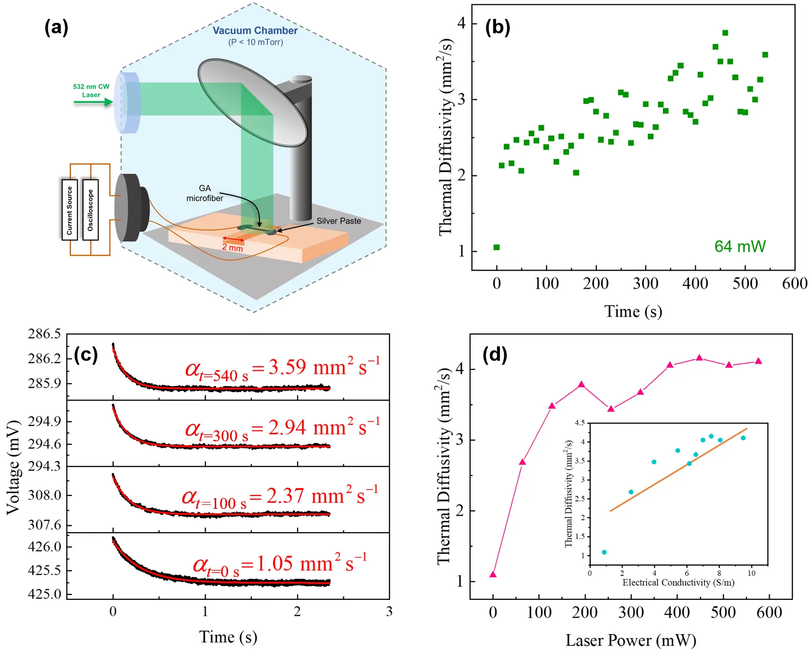
Figure 10. In-situ characterization of the dynamic thermal and electrical behaviors of GA microfibers during CW laser photoreduction by using the TET technique. (a) The schematic of experimental setup; (b) Evolution of thermal diffusivity with time during photoreduction at 64 Mw; (c) Some representative TET signals and fitting during photoreduction; (d) Evolution of thermal diffusivity with the increased laser power recorded at t = 300 s. A linear relationship between electrical conductivity and thermal diffusivity of GA microfibers during photoreduction is presented in the inset^[18]. GA: graphene aerogel; CW: continuous wave; TET: Transient Electro-Thermal.

For composite materials composed of multiple morphologies, phases, or extensive interfaces, thermal conduction behavior becomes significantly more complex, resulting in unique macroscopic thermal and electrical properties. The TET technique serves as an advanced tool for studying transient thermal and electrical responses, offering critical insights into the dynamic evolution of micro- and nanostructures. Xie et al.^[47] discovered an intriguing dual-pace thermal response (DTR) phenomenon in CNT bundles using the TET technique. Figure 11a and Figure 11b illustrate the experimental setup for thermal characterization of a CNT bundle sample. Figure 11c presents a typical V-t curve of the CNT bundle obtained at an environmental temperature of 295 K, which was well fitted using Eq. (6) to extract the thermal diffusivity. When the environmental temperature was lowered to 35 K, the DTR phenomenon appeared in the TET signals (Figure 11d), characterized by a V-t curve comprising a fast-decreasing segment followed by a slow-decreasing segment. This abnormal DTR signal could not be accurately modeled by the conventional TET approach. Instead, a dual-α TET model was developed to fit the DTR data^[21,47]:

Display Full Size

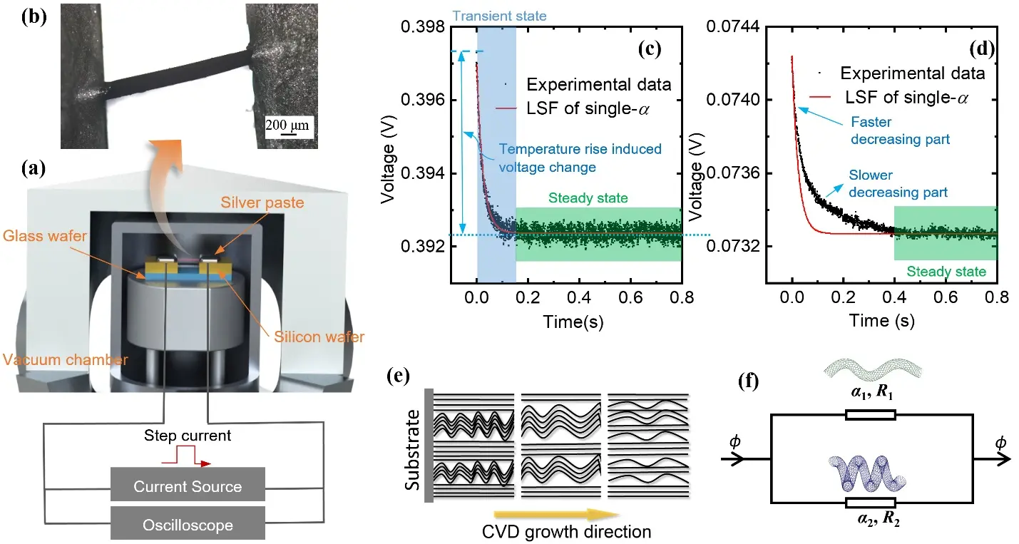
Figure 11. The DTR phenomenon in CNT bundles was discovered based on the TET technique. (a) Schematic of the TET setup; (b) A suspended CNT bundle sample; (c) A typical V-t curve of the CNT bundle obtained at 295 K, which was fitted well based on Eq. (6) to obtain the thermal diffusivity; (d) A DTR phenomenon found in TET signals as the environmental temperature was reduced to 35 K, where the V-t curve became a combination of a fast-decreasing part and a slow-decreasing part; (e) A mixed morphology of straight and coiled CNTs within the bundle resulted from CVD growth; (f) The parallel heat transfer model in the VACNTs arrays after structure separation, which was responsible for the observed DTR phenomenon^[47]. DTR: dual-pace thermal response; CNT: carbon nanotube; TET: Transient Electro-Thermal; CVD: chemical vapor decomposition; VACNTs: vertically aligned carbon nanotube arrays.

(25)$T^{\ast }=A{e}^{-9.911\times {\alpha }_{1}t/L^2}+B{e}^{-9.911\times {\alpha }_{2}t/L^2}+C$

In this model, α₁ and α₂ represent two distinct thermal diffusivities corresponding to simultaneous heat conduction pathways in CNT bundles, arising from the presence of straight CNTs and coiled CNTs within the structure. Figure 11e shows that during CVD growth, a portion of initially straight CNTs transformed into coiled morphologies, resulting in a mixed configuration of straight and coiled CNTs. Combined structural analysis and TET measurements indicate that the observed DTR phenomenon originates from these dual parallel heat conduction pathways, with straight and coiled CNTs functioning as separate phonon transport channels (Figure 11f). The nanoscale structural separation induced by cryogenic thermal strain is responsible for this behavior. This study demonstrates that the coexistence of two CNT morphologies and subsequent nanoscale separation significantly influences both thermal and electrical transport properties in CVD-grown CNT arrays, particularly their transient response characteristics. Such dynamic phenomena are challenging to capture using conventional thermal characterization techniques, especially steady-state measurement methods.

6. Zero Temperature-Rise Limit Measurement: Ultimate Accuracy

In typical TET measurements, a finite temperature rise is necessary to generate a detectable and reliable V-t response. Generally, a minimum relative voltage change of about 0.3% is required for acceptable sensitivity, corresponding to a temperature increase of at least 1K during the test. However, at cryogenic temperatures (e.g., below 50 K), the electrical resistance of metals exhibits minimal variation with temperature. Consequently, achieving the same ~0.3% voltage change requires a much larger temperature rise, often in the range of 20-30 K. This significant temperature rise complicates accurate determination of the true thermal diffusivity (α) at the intended ambient temperature, since the actual measurement occurs at an elevated effective temperature due to Joule heating during I application. To address this challenge and accurately determine α at the designated ambient temperature, a zero temperature-rise approach has been proposed^[27]. In this method, multiple TET measurements are performed at a given ambient temperature using different step currents. These currents produce a range of heating powers (VI), resulting in varying temperature rises and corresponding voltage changes (typically between ~0.3% and ~1.5%). For each ambient temperature, α is determined and then plotted against VI. The resulting plot exhibits a clear linear relationship, where the intercept of the linear fit represents the true α value at zero temperature rise (α₀), i.e., at the actual ambient temperature without Joule heating. This method, introduced in our recent work^[27] enables accurate extrapolation of α to the desired temperature condition.

For a single-walled carbon nanotube (SWCNT) film, the zero temperature-rise method was applied to precisely determine α under ambient and cryogenic conditions^[27]. TET signals of the SWCNT film at different ambient temperatures are shown in Figure 12a, Figure 12b and Figure 12c. At 290 K, the signals were fitted using a single exponential function [Eq.(8)], while two-exponential fitting was required for the 210 K and 170 K signals. Figure 12d, Figure 12e and Figure 12f illustrate the relationship between α and VI at ambient temperatures of 290 K, 210 K, and 170 K, using multiple current levels to produce varying temperature rises. By extrapolating the linear fits to zero power, the α values at the intended ambient temperatures were obtained as 1.92 × 10^-5 m²/s at 290 K, 8.3 × 10^-6 m²/s at 210 K, and 7.93 × 10^-6 m²/s at 170 K.

Display Full Size

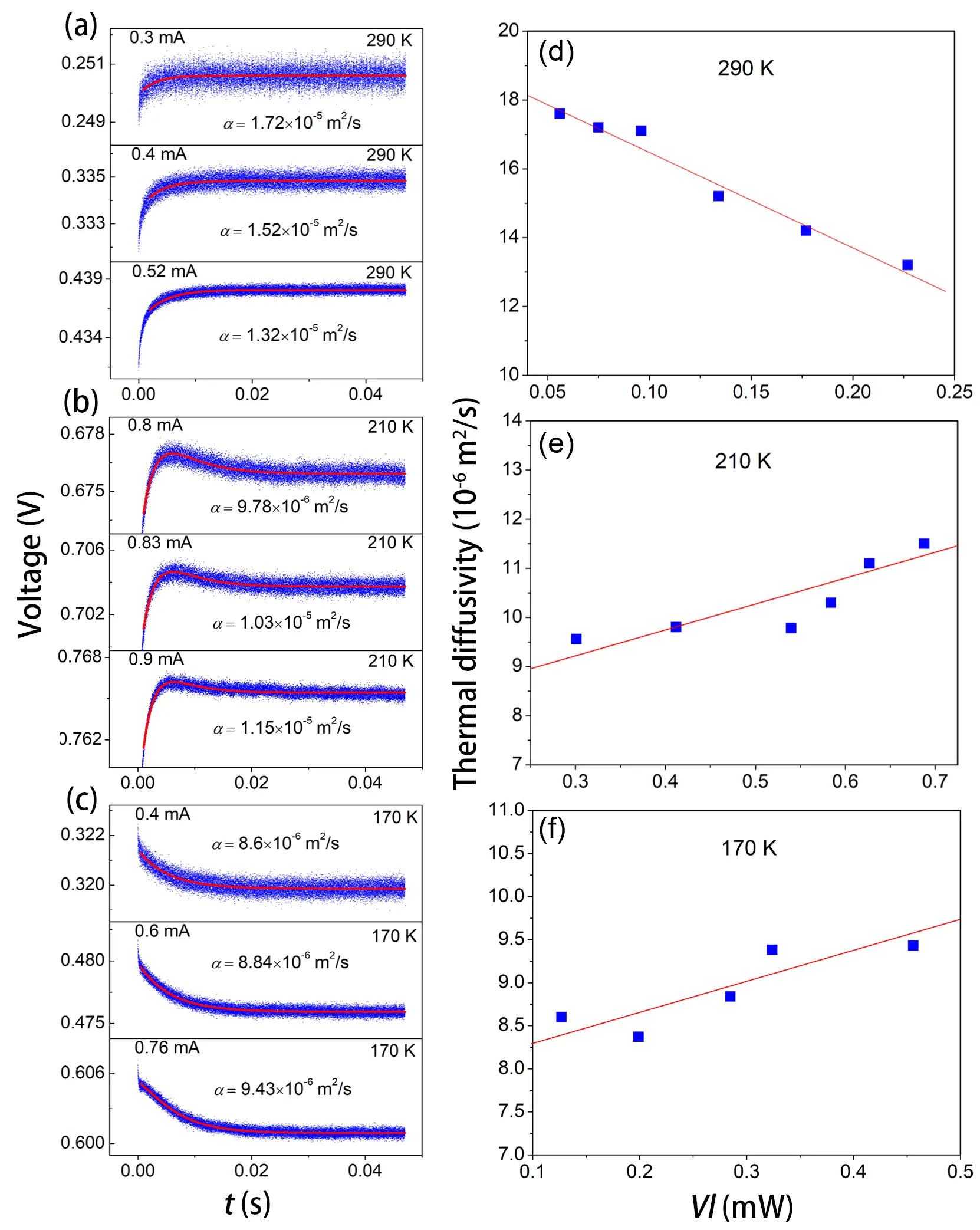
Figure 12. The zero temperature rise method employed to accurately determine the α of a SWCNT film at ambient conditions. The TET signal responses of a SWCNT film subjected to various levels of current-induced heating at (a) 290 K, (b) 210 K, and (c) 170 K; A single-exponential fitting is applied at 290 K, while a two-exponential fitting approach is employed for 210 K and 170 K; Panels (d-f) illustrate how the thermal diffusivity of the SWCNT film changes with heating intensity at each respective temperature^[27]. SWCNT: single-walled carbon nanotube; TET: Transient Electro-Thermal.

As detailed in Section 2.2, TET measurements were also conducted on a microscale platinum wire at four different current levels: 16, 18, 19, and 19.5mA. For each current, 10 repeated measurements were performed to assess reproducibility and current-dependent effects on thermal diffusivity. Figure 3d shows the relationship between measured α and corresponding VI. The solid red markers represent the mean α at each current level, and a linear regression was applied to these values to extrapolate thermal diffusivity at zero power, effectively eliminating Joule heating effects. The intercept of the linear fit yielded α₀ = 2.495 × 10^-5 ± 3.72 × 10^-7 m²/s. For comparison, the average α measured at the lowest current level (16 mA) was 2.295 × 10^-5 m²/s, reflecting an 8.7% difference. Notably, the extrapolated α₀ closely matched the literature value for Pt (2.51 × 10^-5 m²/s), with an excellent agreement of about 0.6%. This confirms the effectiveness of the zero temperature-rise approach in improving measurement accuracy and underscores the importance of correcting for temperature rise effects in high-precision thermal characterization.

Finally, Figure 13 demonstrates the capability of the TET technique to characterize thermal diffusivity of SWCNT films down to cryogenic temperatures^[27]. As shown on the left axis, α decreases steadily from 1.81 × 10^-5 m²/s at 290 K to 5.02 × 10^-6 m²/s at 40K, and then gradually levels off at approximately 4.0 × 10^-6 m²/s at 12 K. This result highlights the robustness of the method in capturing accurate thermal transport properties at temperatures as low as 12 K^[27].

Display Full Size

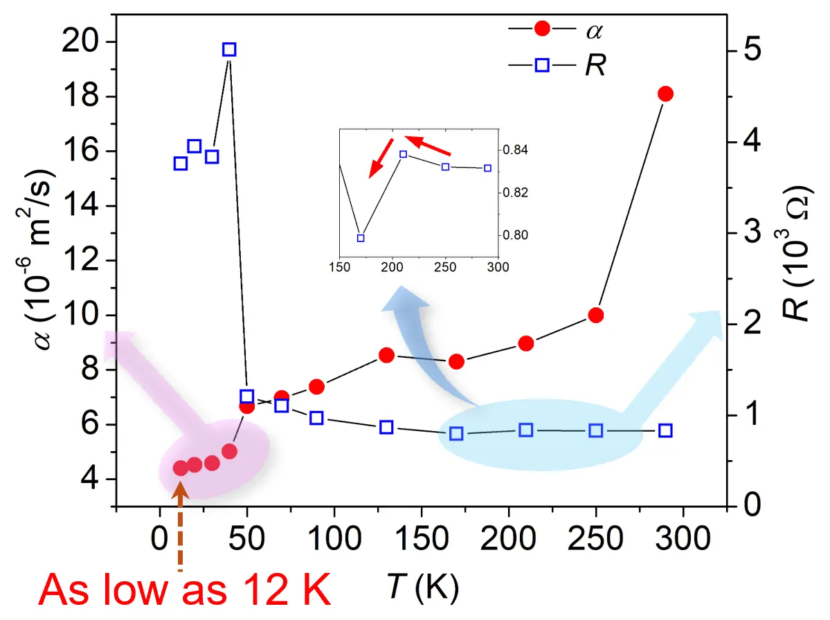
Figure 13. The measured thermal diffusivity (left axis) and electrical resistance (right axis) of the SWCNT film against temperature, demonstrating the effectiveness of the TET technique at very low temperatures, reaching as low as 12 K. The inset highlights the temperature (~210 K) at which the slope of resistance with respect to temperature (θ_T) changes sign^[27]. SWCNT: single-walled carbon nanotube; TET: Transient Electro-Thermal.

7. Concluding Remarks and Outlook

The TET technique offers a rapid and highly accurate approach for measuring the thermal diffusivity and thermal conductivity of 1D materials, whether dielectric, metallic, or semiconductive. In its early development, three specific data analysis methods were introduced: initial-stage linear fitting, the characteristic point method, and the least-squares fitting approach for extracting α_eff. Later, the linear fitting method based on the relation between ln(1-T^*) further simplified the process. With appropriate experimental control, measurement accuracy can reach better than 1%. The TET physical model has been expanded to accommodate nonlinear ρ_e-T behavior, including higher-order dependencies of electrical resistivity on temperature and even reversed signs of θ_T. Furthermore, the zero-temperature-rise strategy enables accurate determination of thermal diffusivity at the designated ambient temperature, which is critical for cryogenic property measurements. Additionally, radiative and convective heat transfer, as well as the effect of metallic coatings, can be quantitatively assessed and removed from α_eff. By varying suspended lengths or coating thicknesses and applying extrapolation, both surface emissivity and the Lorenz number of metallic coatings can be simultaneously determined. The differential TET methodology extends the applicability of the technique to materials thinner than 1nm, enabling high-precision measurements of various 2D materials whose thickness typically ranges from a few nanometers to sub-nanometer scales.

Despite its potential, the differential TET method remains underutilized. We anticipate it will significantly advance the accurate characterization of thermal transport in 2D materials, surpassing Raman spectroscopy-based approaches. Conventional Raman methods require determining the Raman temperature coefficient and the laser absorption rate, parameters that are difficult to measure accurately and often introduce large errors^[48]. Additionally, neglecting optical-acoustic phonon nonequilibrium can lead to substantial overestimation of temperature rise, especially for supported 2D materials. Although advanced methods such as energy transport-state resolved Raman in time (ET-Raman) and frequency domains (FET-Raman)^[49], can mitigate some limitations, their accuracy still does not match that of differential TET when applicable.

TET measurements also provide insights into interfacial thermal resistance (ITR). When a sample is supported on a large substrate, the measured effective thermal diffusivity includes the contribution of ITR. By subtracting in-plane heat transfer along the sample, ITR can be determined with high accuracy. While the 3ω technique can also measure ITR, its implementation and physical modeling are less straightforward compared to TET. Future research in this direction could significantly enhance our understanding of ITR at 1D micro/nanoscale contact lines, an area that remains largely unexplored. Furthermore, zero-dimensional (0D) heat transfer, which refers to heat transfer occurring at the contact point between two non-parallel fibers, has been rarely studied, primarily due to the significant challenges associated with its measurement. The TET technique offers a practical approach for this purpose by comparing the thermal diffusivity of a fiber before (α₁) and after its contact with a second fiber (α₂). Because of the additional heat transfer through the point contact, α₂ should be greater than α₁. With an appropriate physical model, the ITR at the contact can be accurately determined^[50]. This type of 0D heat transfer is of great interest since bundles consisting of micro/nanoscale fibers/wires will have abundant point contacts between fibers/wires, and such contacts in fact play a critical role in the overall thermal conductivity of the material.

Dynamic thermal characterization is essential for understanding time-dependent thermal behavior in chemical processes and material treatments involving transient heat transfer, phase transitions, or microstructural evolution. With its excellent temporal resolution (typically < 1 s per measurement), the TET technique is a powerful tool for real-time characterization of dynamic thermophysical properties. Previous studies have demonstrated its use in monitoring thermal annealing and photoreduction of carbon materials, as well as biomass pyrolysis. Looking ahead, integrating dynamic TET characterization with chemical processes and material treatment platforms could provide transformative insights into phase transitions and microstructure evolution. Potential applications include phase-change fibers and films for adaptive thermal management, polymer curing for aerospace and automotive components, and laser sintering or melting in metal additive manufacturing. To support these applications, new physical models must account for latent heat during phase-change characterization. Additionally, strain-thermal correlations, critical for the reliability and performance of flexible electronics, can be explored using dynamic TET. These capabilities open new pathways for advancing material science, optimizing manufacturing processes, and improving device performance, with promising applications in energy storage, thermal management, and advanced manufacturing.

Authors contribution

Xie Y: Funding acquisition, investigation, writing, writing-review & editing.

Karamati A: Data curation and formal analysis, investigation, writing.

Wang X: Conceptualization, data curation and formal analysis, investigation, project administration and supervision, writing, writing-review & editing.

Conflicts of interest

Xinwei Wang is an Editorial Board member of Thermo-X. The other authors declare no conflicts of interest.

Ethical approval

Not applicable.

Consent to participate

Not applicable

Consent for publication

Not applicable.

Availability of data and materials

Not applicable.

Funding

The work was supported by the National Natural Science Foundation of China (No. 52276080, No. U23A20111, and 52411540235 for Y. Xie).

Copyright

© The Author(s) 2025.

References

-
1. Wang X, Xu X, Choi SUS. Thermal conductivity of nanoparticle-fluid mixture. J Thermophys Heat Transf. 1999;13(4):474-480.
[DOI] -
2. Li D, Wu Y, Fan R, Yang P, Majumdar A. Thermal conductivity of Si/SiGe superlattice nanowires. Appl Phys Lett. 2003;83(15):3186-3188.
3. Assael MJ, Antoniadis KD, Wakeham WA. Historical evolution of the transient hot-wire technique. Int J Thermophys. 2010;31(6):1051-1072.
4. Assael MJ, Antoniadis KD, Velliadou D, Wakeham WA. Correct use of the transient hot-wire technique for thermal conductivity measurements on fluids. Int J Thermophys. 2023;44(6):85.
5. Parker WJ, Jenkins RJ, Butler CP, Abbott GL. Flash method of determining thermal diffusivity, heat capacity, and thermal conductivity. J Appl Phys. 1961;32(9):1679-1684.
6. Liu J, Han M, Wang R, Xu S, Wang X. Photothermal phenomenon: Extended ideas for thermophysical properties characterization. J Appl Phys. 2022;131(6):065107.
7. Cahill DG, Allen TH. Thermal conductivity of sputtered and evaporated SiO2 and TiO2 optical coatings. Appl Phys Lett. 1994;65:309-311.
8. Cahill DG, Ford WK, Goodson KE, Mahan GD, Majumdar A, Maris HJ, et al. Nanoscale thermal transport. J Appl Phys. 2003;93(2):793-818.
9. Zheng Q, Kaur S, Dames C, Prasher R S. Analysis and improvement of the hot disk transient plane source method for low thermal conductivity materials. Int J Heat Mass Transf. 2020;151:119331.
10. He Y. Rapid thermal conductivity measurement with a hot disk sensor: Part 1. Theoretical considerations. Thermochim Acta. 2005;436(1-2):122-129.
11. Landry D, Flores R, Goodman RB. Estimating the thermal conductivity of thin films: A novel approach using the transient plane source method. J Heat Mass Transfer Mar. 2024;146(3):031004.
12. Gu J, Safiullah SB, Yang L, Qian Z, Zheng Q. Improving the accuracy of transient plane source thermal conductivity measurements: Novel analytical models, fitting approaches, and systematic sensitivity analysis. Int J Heat Mass Transf. 2025;247:27110.
13. Wang D, Ban H, Jiang P. Three-dimensional (3D) tensor-based methodology for characterizing 3D anisotropic thermal conductivity tensor. Int J Heat Mass Transf. 2025;242:126886.
14. Guo JQ, Wang XW, Wang T. Thermal characterization of microscale conductive and nonconductive wires using transient electrothermal technique. J Appl Phys. 2007;101(6):063537.
15. Bai J, Karamati A, Duan X, Lin H, Wang X. Structure thermal domain size in μm-thick single crystalline sapphire wafer uncovered by low-momentum phonon scattering. J Phys Chem C. 2025;129(11):5754-5761.
16. Karamati A, Deng C, Qu W, Bai X, Xu S, Eres G, et al. Temperature dependence of resistivity of carbon micro/nanostructures: Microscale spatial distribution with mixed metallic and semiconductive behaviors. J Appl Phys. 2023;134(8):085102.
17. Alahmad Q, Rahbar M, Karamati A, Bai J, Wang X. 3D strongly anisotropic intrinsic thermal conductivity of polypropylene separator. J Power Sources. 2023;580:233377.
18. Hunter N, Karamati A, Xie Y, Lin H, Wang X. Laser photoreduction of graphene aerogel microfibers: Dynamic electrical and thermal behaviors. ChemPhysChem. 2022;23(23):e202200417.
19. Xu S, Zobeiri H, Hunter N, Zhang H, Eres G, Wang X. Photocurrent in carbon nanotube bundle: Graded Seebeck coefficient phenomenon. Nano Energy. 2021;86:106054.
20. Wang R, Zobeiri H, Lin H, Qu W, Bai X, Deng C, Wang X. Anisotropic thermal conductivities and structure in lignin-based microscale carbon fibers. Carbon. 2019;147:58-69.
21. Xie Y, Yuan P, Wang T, Hashemi N, Wang X. Switch on the high thermal conductivity of graphene paper. Nanoscale. 2016;8 (40):17581-17597.
22. Guo J, Wang X, Zhang L, Wang T. Transient thermal characterization of micro/submicroscale polyacrylonitrile wires. Appl Phys. 2007;89:153-156.
23. Deng C, Sun Y, Pan L, Wang T, Xie Y, Liu J, et al. Thermal diffusivity of a single carbon nanocoil: Uncovering the correlation with temperature and domain size. ACS Nano. 2016;10(10):9710-9719.
24. Zhu B, Wang R, Harrison S, Williams K, Goduguchinta R, Schneiter J, et al. Thermal conductivity of SiC microwires: Effect of temperature and structural domain size uncovered by 0 K limit phonon scattering. Ceram Int. 2018;44(10):11218-11224.
25. Xie Y, Wang T, Zhu B, Yan C, Zhang P, Wang X, et al. 19-Fold thermal conductivity increase of carbon nanotube bundles toward high-end thermal design applications. Carbon. 2018;139:445-458.
26. Alahmad Q, Rahbar M, Han M, Lin H, Xu S, Wang X. Thermal conductivity of gas diffusion layers of PEM fuel cells: Anisotropy and effects of structures. Int J Thermophys. 2023;44(11):167.
27. Karamati A, Han M, Duan X, Xie Y, Wang X. Thermal diffusivity characterization of semiconductive 1D micro/nanoscale structures. Int J Heat Mass Transf. 2024;233:126012.
28. Karamati A, Hunter N, Lin H, Zobeiri H, Xu S, Wang X. Strong linearity and effect of laser heating location in transient photo/electrothermal characterization of micro/nanoscale wires. Int J Heat Mass Transf. 2022;198:123393.
29. Bates DM, Watts DG. Nonlinear regression analysis and its applications. New York: Wiley; 1988.
30. Guo J, Wang X, Geohegan DB, Eres G, Vincent C. Development of pulsed laser-assisted thermal relaxation technique for thermal characterization of microscale wires. J Appl Phys. 2008;103(11):113505.
31. Lin H, Xu S, Wang XW, Mei N. Significantly reduced thermal diffusivity of free-standing two-layer graphene in graphene foam. Nanotechnology. 2013;24(41):415076.
32. Xie Y, Xu Z, Xu S, Cheng Z, Hashemi N, Deng C, et al. The defect level and ideal thermal conductivity of graphene uncovered by residual thermal reffusivity at the 0 K limit. Nanoscale. 2015;7 (22):10101-10110.
33. Xie Y, Xu S, Xu Z, Wu H, Deng C, Wang X. Interface-mediated extremely low thermal conductivity of graphene aerogel. Carbon. 2016;98:381-390.
34. Huang Y, Wei L, Chen T, Xu T, Cai Y, Guo Y, et al. Ultra-low-density carbon nanotube aerogel film for fast and sensitive bolometric sensing. Acs Appl Mater Inter 2023;15(9):12137-12145.
35. Liu J, Wang T, Xu S, Yuan P, Xu X, Wang X. Thermal conductivity of giant mono- to few-layered CVD graphene supported on an organic substrate. Nanoscale. 2016;8(19):10298-10309.
36. Lin H, Xu S, Wang X, Mei N. Thermal and electrical cnduction in ultrathin metallic films: 7 nm down to sub-nanometer thickness. Small. 2013;9(15):2585-2594.
37. Lin H, Xu S, Li C, Dong H, Wang X. Thermal and electrical conduction in 6.4 nm thin gold films. Nanoscale. 2013;5(11):4652-4656.
38. Gao J, Zobeiri H, Lin H, Xie D, Yue Y, Wang X. Coherency between thermal and electrical transport of partly reduced graphene paper. Carbon. 2021;178:92-102.
39. Xie Y, Wang X. Thermal conductivity of carbon-based nanomaterials: Deep understanding of the structural effects. Green Carbon. 2023;1(1):47-57.
40. Lin H, Xu S, Zhang YQ, Wang X. Electron transport and bulk-like behavior of wiedemann-franz law for sub-7 nm-thin iridium films on silkworm silk. ACS Appl Mater Interfaces. 2014;6(14):11341-11347.
41. Cheng Z, Xu Z, Xu S, Wang X. Phonon softening and weak temperature-dependent lorenz number for bio-supported ultra-thin Ir film. arXiv preprint arXiv: 1410.1912 [Preprint]. 2014.
42. Cheng Z, Xu Z, Xu S, Wang X. Temperature dependent behavior of thermal conductivity of sub-5 nm Ir film: Defect-electron scattering quantified by residual thermal resistivity. J Appl Phys. 2015;117(2):024307.
43. Alahmad Q, Lin H, Liu J, Rahbar M, Kingston TA, Wang X. Characterization of the in-plane thermal conductivity of sub-10 nm Ir films on a flexible substrate. Int J Thermophys. 2025;46:141.
44. Xu Z, Wang X, Xie H. Promoted electron transport and sustained phonon transport by DNA down to 10 K. Polymer. 2014;55(24):6373-6380.
45. Liu J, Qu W, Xie Y, Zhu B, Wang T, Bai X, et al. Thermal conductivity and annealing effect on structure of lignin-based microscale carbon fibers. Carbon. 2017;121:35-47.
46. Xu C, Xu S, Zhang Z, Lin H. Research on in situ thermophysical properties measurement during heating processes. Nanomaterials. 2023;13(1):119.
47. Xie Y, Zobeiri H, Xiang L, Eres G, Wang J, Wang X. Dual-pace transient heat conduction in vertically aligned carbon nanotube arrays induced by structure separation. Nano Energy. 2021;90:106516.
48. Xu S, Fan A, Wang H, Zhang X, Wang X. Raman-based nanoscale thermal transport characterization: A critical review. Int J Heat Mass Transf. 2020;154:119751.
49. Wang R, Hunter N, Zobeiri H, Xu S, Wang X. Critical problems faced in Raman-based energy transport characterization of nanomaterials. Phys Chem Chem Phys. 2022;24(37):22390-22404.
50. Van Velson N, Wang X. Characterization of thermal transport across single-point contact between micro-wires. Appl Phys A. 2013;110(2):403-412.
[DOI]
Copyright
© The Author(s) 2025. This is an Open Access article licensed under a Creative Commons Attribution 4.0 International License (https://creativecommons.org/licenses/by/4.0/), which permits unrestricted use, sharing, adaptation, distribution and reproduction in any medium or format, for any purpose, even commercially, as long as you give appropriate credit to the original author(s) and the source, provide a link to the Creative Commons license, and indicate if changes were made.
Publisher’s Note
Science Exploration remains a neutral stance on jurisdictional claims in published
maps
and institutional affiliations. The views expressed in this article are solely those
of
the author(s) and do not reflect the opinions of the Editors or the publisher.
Share And Cite
Science Exploration Style
Xie Y, Karamati A, Wang X. Transient electro-thermal technique for measuring the thermal diffusivity/conductivity of 1D/2D materials: from mm down to atomic scale thickness. Thermo-X. 2025;1:202503. https://doi.org/10.70401/tx.2025.0002
Tips
Copy completed.
Submit a Manuscript
Author Instructions
Cite this Article
Article Metrics
0
View
Download
Article Updates